Chapter 11: Bayesian Model Selection in Regression and Time Series Analysis
Chapter11.RmdSection 11.4: Model Selection Problems in Time Series Analysis
Section 11.4.1: Selecting the model order in an AR(p) model
Akin to Chapter 7, we load the US GDP data, restrict our analysis to the time before the COVID outbreak, and compute log returns.
data("gdp", package = "BayesianLearningCode")
dat <- gdp[1:which(names(gdp) == "2019-10-01")]
logret <- log(dat[-1]) - log(dat[-length(dat)])
logret <- ts(logret, start = c(1947, 2), end = c(2019, 4),
             frequency = 4)
We re-use the regression function defined in Chapter 7, again using the tools developed in Chapter 6. In addition, we store the parameters of the conditional posteriors to compute Savage-Dickey density ratios and marginal likelihoods at a later stage.
library("BayesianLearningCode")
library("mvtnorm")

regression <- function(y, X, b0, B0, c0, C0,
                       nburn = 1000L, M = 100000L / mcmcspeedup) {

  N <- nrow(X)
  d <- ncol(X)

  if (length(b0) == 1L) b0 <- rep(b0, d)

  if (!is.matrix(B0)) {
    if (length(B0) == 1L) {
      B0 <- diag(rep(B0, d))
    } else {
      B0 <- diag(B0)
    }
  }

  # Precompute some values
  B0inv <- solve(B0)
  B0invb0 <- B0inv %*% b0
  cN <- c0 + N / 2
  XX <- crossprod(X)
  Xy <- crossprod(X, y)

  # Prepare memory to store the draws
  betas <- matrix(NA_real_, nrow = M, ncol = d)
  sigma2s <- rep(NA_real_, M)
  colnames(betas) <- colnames(X)

  # Prepare memory to store the parameters
  paras <- list(bN = matrix(NA_real_, nrow = M, ncol = d),
                BN = array(NA_real_, dim = c(M, d, d)),
                cN = rep(NA_real_, M),
                CN = rep(NA_real_, M))

  # Set the starting value for beta
  sigma2 <- var(y) / 2

  # Run the Gibbs sampler
  for (m in seq_len(nburn + M)) {
    # Sample beta from its full conditional
    BN <- solve(B0inv + XX / sigma2)
    bN <- BN %*% (B0invb0 + Xy / sigma2)
    beta <- rmvnorm(1, mean = bN, sigma = BN)

    # Sample sigma^2 from its full conditional
    eps <- y - tcrossprod(X, beta)
    CN <- C0 + crossprod(eps) / 2
    sigma2 <- rinvgamma(1, cN, CN)

    # Store the results
    if (m > nburn) {
      betas[m - nburn, ] <- beta
      sigma2s[m - nburn] <- sigma2
      paras[["bN"]][m - nburn, ] <- bN
      paras[["BN"]][m - nburn, , ] <- BN
      paras[["cN"]][m - nburn] <- cN
      paras[["CN"]][m - nburn] <- CN
    }
  }
  list(betas = betas, sigma2s = sigma2s, paras = paras, X = X, y = y,
       b0 = b0, B0 = B0, c0 = c0, C0 = C0)
}
We also need a function to create the AR-specific design matrix (also re-used from Chapter 7, now with the added option to condition on more initial data than then bare minimum).
ARdesignmatrix <- function(dat, p = 1, conditioninglength = p) {
  d <- p + 1
  N <- length(dat) - p

  Xy <- matrix(NA_real_, N, d)
  Xy[, 1] <- 1
  for (i in seq_len(p)) {
    Xy[, i + 1] <- dat[(p + 1 - i) : (length(dat) - i)]
  }
  Xy[(1 + conditioninglength - p):N, , drop = FALSE]
}
Now we are ready to reproduce the results in the book.
Example 11.8: US GDP data: Choosing the model order via Savage-Dickey density ratios
We obtain draws and parameters for four AR models under the semi-conjugate prior.
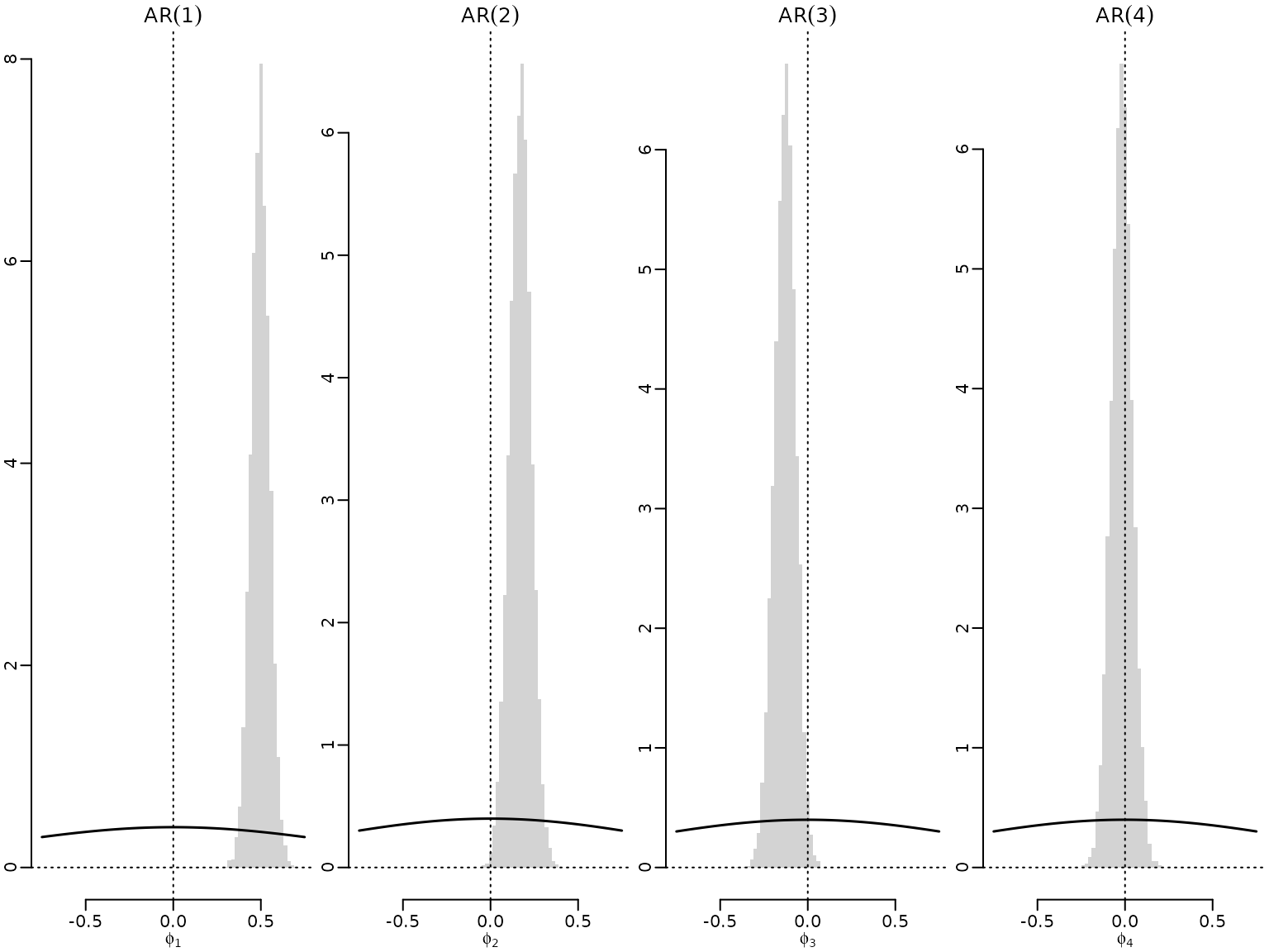
Figure 11.2: Graphical assessment of the Savage-Dickey density ratio
Now we plot the draws for the leading coefficient, i.e., the coefficient corresponding to the highest lag in each of the models, along with the marginal prior.
mymin <- -.75
mymax <- .75
mybreaks <- seq(mymin, mymax, by = .02)
myats <- seq(mymin, mymax, length.out = 200)
for (i in 2:5) {
  p <- i - 1
  hist(res[[i]]$betas[, p + 1], freq = FALSE, main = bquote(AR(.(p))),
       xlab = bquote(phi[.(p)]), ylab = "", breaks = mybreaks, border = NA)
  abline(v = 0, lty = 3)
  abline(h = 0, lty = 3)
  lines(myats, dnorm(myats, b0, sqrt(B0)), lwd = 1.5)
}
After visualizing the Savage-Dickey density ratio, we now move towards computing its numerical value by Rao-Blackwellization. We first define a numerically stable version of the log-sum-exp (log-mean-exp) function.
logsumexp <- function(x) {
  maxx <- max(x)
  maxx + log(sum(exp(x - maxx)))
}

logmeanexp <- function(x) {
  logsumexp(x) - log(length(x))
}
Now we are ready to compute.
logSD <- rep(NA_real_, length(res) - 1)
for (i in seq_len(length(res) - 1)) {
  p <- i
  means <- res[[i + 1]]$paras$bN[, p + 1]
  sds <- sqrt(res[[i + 1]]$paras$BN[, p + 1, p + 1])
  logSD[i] <- logmeanexp(dnorm(0, means, sds, log = TRUE)) -
    dnorm(0, b0, sqrt(B0), log = TRUE)
}
names(logSD) <- c("0 vs 1", "1 vs 2", "2 vs 3", "3 vs 4")
round(logSD, 2)
#> 0 vs 1 1 vs 2 2 vs 3 3 vs 4
#> -35.98  -1.18   0.46   2.75
Note that the first value of logSD is numerically rather unstable.
To reproduce this using Chib’s method, we need to be careful to compare models which were estimated conditional on the same initial data. Thus, we re-estimate conditioning on one extra initial observation.
set.seed(seed)
res2 <- vector("list", 5)
for (i in seq_along(res2)) {
  p <- i - 1
  y <- tail(logret, -(p + 1))
  Xy <- ARdesignmatrix(logret, p, conditioninglength = p + 1)
  res2[[i]] <- regression(y, Xy, b0 = b0, B0 = B0, c0 = 2, C0 = 0.001)
}
And now, we always condition on the first four observations (irrespectively of the model order). This makes it possible to compare all AR models via model probabilities.
set.seed(seed)
res3 <- vector("list", 5)
for (i in seq_along(res3)) {
  p <- i - 1
  y <- tail(logret, -4)
  Xy <- ARdesignmatrix(logret, p, conditioninglength = 4)
  res3[[i]] <- regression(y, Xy, b0 = b0, B0 = B0, c0 = 2, C0 = 0.001)
}
We now compute Chib’s estimator, evaluated at the posterior median.
allres <- list(res, res2, res3)
logML <- matrix(NA_real_, length(allres), length(res))
for (i in seq_along(allres)) {
  for (j in seq_len(length(res))) {
    myres <- allres[[i]][[j]]
    beta_med <- apply(myres$betas, 2, median)
    sigma2_med <- median(myres$sigma2s)
    BN_med <- solve(solve(myres$B0) + crossprod(myres$X) / sigma2_med)
    bN_med <- BN_med %*% (solve(myres$B0) %*% myres$b0 +
                            crossprod(myres$X, myres$y) / sigma2_med)
    logML[i, j] <-
      sum(dnorm(myres$y, myres$X %*% beta_med, sqrt(sigma2_med), log = TRUE)) +
      dmvnorm(beta_med, myres$b0, myres$B0, log = TRUE) +
      dinvgamma(sigma2_med, myres$c0, myres$C0, log = TRUE) -
      dmvnorm(beta_med, bN_med, BN_med, log = TRUE) -
      logmeanexp(dinvgamma(sigma2_med, myres$paras$cN, myres$paras$CN, log = TRUE))
  }
}
dimnames(logML) <- list("Conditioning set length" = c("p", "p + 1", "4"),
                        "Lag order" = seq_len(ncol(logML)))
knitr::kable(round(logML, 2))| 1 | 2 | 3 | 4 | 5 | |
|---|---|---|---|---|---|
| p | 890.93 | 923.38 | 920.86 | 920.21 | 913.80 |
| p + 1 | 887.41 | 919.68 | 920.68 | 916.56 | 910.09 |
| 4 | 879.34 | 915.67 | 916.99 | 916.56 | 913.80 |
The values below should be equal to the logSD values from above.
pairwiselogML <- logML[2, 1:4] - logML[1, 2:5]
names(pairwiselogML) <- names(logSD)
round(pairwiselogML, 2)
#> 0 vs 1 1 vs 2 2 vs 3 3 vs 4
#> -35.97  -1.18   0.47   2.75
To compute model probabilities, we use the uniform and the penalty prior.
# Uniform prior:
stableML <- exp(logML[3, ] - max(logML[3, ]))
probs_unif <- stableML / sum(stableML)

# Penalty prior:
tmp <- logML[3, ] - log(seq_along(stableML)) - log(seq_along(stableML) + 1)
stablepost <- exp(tmp - max(tmp))
probs_pen <- stablepost / sum(stablepost)

knitr::kable(t(round(cbind(unif = probs_unif, penalized = probs_pen), 3)))| 1 | 2 | 3 | 4 | 5 | |
|---|---|---|---|---|---|
| unif | 0 | 0.136 | 0.512 | 0.331 | 0.021 |
| penalized | 0 | 0.275 | 0.516 | 0.200 | 0.009 |
Example 11.18: Application to Austrian wage mobility data - homogeneity versus grouped model
We load the data and reduce the observations to workers from the birth cohort 1946-1960.
data("labor", package = "BayesianLearningCode")
labor <- subset(labor, birthyear >= 1946 & birthyear <= 1960)
We extract the income columns and transform the data to obtain for each worker the matrix which contains the number of transitions from one class to the other, i.e., the matrix with values .
income <- labor[, grepl("^income", colnames(labor))]
income <- sapply(income, as.integer)
colnames(income) <- gsub("income_", "", colnames(income))
getTransitions <- function(x, classes) {
    transitions <- matrix(0, length(classes), length(classes))
    for (i in seq_len(length(x) - 1)) {
        transitions[x[i], x[i + 1]] <- transitions[x[i], x[i + 1]] + 1
    }
    dimnames(transitions) <- list(from = classes, to = classes)
    transitions
}
income_transitions <-
    lapply(seq_len(nrow(income)),
           function(i) getTransitions(income[i, ], classes = 0:5))
We determine the marginal likelihood of the first-order Markov chain model assuming homogeneity and grouping by gender.
N_hk <- Reduce("+", income_transitions)
Ng_hk <- list(male = Reduce("+", income_transitions[!labor$female]),
              female = Reduce("+", income_transitions[labor$female]))
gammas <- c(1, 4)
K <- nrow(N_hk)
G <- length(Ng_hk)
logmarglikMH <- logmarglikMG <- numeric(2)
for (i in 1:2) {
    gamma <- gammas[i]
    logmarglikMH[i] <- K * (lgamma(K * gamma) - K * lgamma(gamma)) +
        sum(lgamma(gamma + N_hk)) -
        sum(lgamma(rowSums(gamma + N_hk)))
    logmarglikMG[i] <- G * K * (lgamma(K * gamma) - K * lgamma(gamma)) +
        sum(lgamma(gamma + Ng_hk[["male"]])) +
        sum(lgamma(gamma + Ng_hk[["female"]])) -
        sum(lgamma(rowSums(gamma + Ng_hk[["male"]]))) -
        sum(lgamma(rowSums(gamma + Ng_hk[["female"]])))
}
We also calculate the log BF and summarize results.
res <- rbind(MH = c(logmarglikMH, NA, NA),
             MG = c(logmarglikMG, logmarglikMG - logmarglikMH))
colnames(res) <- c("gamma = 1", "gamma = 4",
                   "gamma = 1", "gamma = 4")
knitr::kable(res)| gamma = 1 | gamma = 4 | gamma = 1 | gamma = 4 | |
|---|---|---|---|---|
| MH | -13887.79 | -14030.63 | NA | NA |
| MG | -13833.11 | -14096.42 | 54.68241 | -65.79208 |
Example 11.19: Application to Austrian wage mobility data - restricted models
We continue to compare restricted models to the grouped model. We first calculate the log BFs for the restricted models.
logBF_R1G <- logBF_R2G <- numeric(2)
for (i in 1:2) {
    gamma <- gammas[i]
    logBF_R1G[i] <- lbeta(gamma, gamma) -
        lbeta(gamma + Ng_hk[["male"]]["1", "0"],
              gamma + Ng_hk[["male"]]["1", "2"])
    aN1 <- gamma + Ng_hk[["male"]]["1", "0"]
    aN2 <- gamma + Ng_hk[["female"]]["1", "0"]
    bN1 <- sum(gamma + Ng_hk[["male"]]["1", -1])
    bN2 <- sum(gamma + Ng_hk[["female"]]["1", -1])
    logBF_R2G[i] <- lbeta(aN1 + aN2 - 1, bN1 + bN2 - 1) +
        2 * lbeta(gamma, (K - 1) * gamma) -
        lbeta(aN1, bN1) - lbeta(aN2, bN2) -
        lbeta(2 * gamma - 1, 2 * (K - 1) * gamma - 1)
}
We obtain the log marginal likelihoods for the restricted models from the log marginal likelihoods of the grouped models and the log BFs. We then also summarize the results.
logmarglikR1 <- logmarglikMG + logBF_R1G
logmarglikR2 <- logmarglikMG + logBF_R2G
res <- rbind(MR1 = c(logmarglikR1, logBF_R1G),
             MR2 = c(logmarglikR2, logBF_R2G))
colnames(res) <- c("gamma = 1", "gamma = 4",
                   "gamma = 1", "gamma = 4")
knitr::kable(res)| gamma = 1 | gamma = 4 | gamma = 1 | gamma = 4 | |
|---|---|---|---|---|
| MR1 | -13708.76 | -13972.84 | 124.3463 | 123.580533 |
| MR2 | -13838.72 | -14102.41 | -5.6139 | -5.990161 |