Chapter 1: From Bayes’ Rule to Bayes’ Theorem • BayesianLearningCode

Section 1.3: Naive Bayes classifiers

Example 1.3 and 1.4: Classifying categorical observations into two states

We have two firms, a reliable firm $A$ with $Pr(A) = 0.7$ and a less reliable firm $A^C$ with $Pr(A^C) = 1 - 0.7 = 0.3$ .

PrA <- 0.7
PrAC <- 1 - PrA

The failure rate, i.e., the probability of a faulty item, is 0.01 for the reliable firm $A$ and 0.05 for the less reliable firm $A^C$ .

PrFA <- 0.01
PrFAC <- 0.05

Assume that we observe any number of failures $y$ between 0 and 6 (from $N = 100$ observations in total), but we don’t know whether the items are from company $A$ or $A^C$ .

N <- 100
y <- 0:6

We can now compute the probability of dealing with items from company $A$ by using Bayes’ theorem.

theta1_y_unnormalized <- PrFA ^ y * (1 - PrFA) ^ (N - y) * PrA
theta0_y_unnormalized <- PrFAC ^ y * (1 - PrFAC) ^ (N - y) * PrAC
normalizer <- theta1_y_unnormalized + theta0_y_unnormalized

res <- rbind("reliable company" = theta1_y_unnormalized / normalizer,
             "less reliable company" = theta0_y_unnormalized / normalizer)
colnames(res) <- y
knitr::kable(round(res, 3))

	0	1	2	3	4	5	6
reliable company	0.993	0.965	0.842	0.505	0.164	0.036	0.007
less reliable company	0.007	0.035	0.158	0.495	0.836	0.964	0.993

Note that, of course, the probabilities of dealing with items from company $A$ and $A^C$ are complementary (i.e., sum to one).

Assuming we do not have any prior information about the probability of occurrence of company $A$ , we could simply set $Pr(A) = Pr(A^C) = 0.5$ and recompute the posterior probabilities.

PrA <- 0.5
PrAC <- 1 - PrA

theta1_y_unnormalized <- PrFA ^ y * (1 - PrFA) ^ (N - y) * PrA
theta0_y_unnormalized <- PrFAC ^ y * (1 - PrFAC) ^ (N - y) * PrAC
normalizer <- theta1_y_unnormalized + theta0_y_unnormalized

res <- rbind(theta1_y_unnormalized/ normalizer,
             theta0_y_unnormalized/ normalizer)
colnames(res) <- y
rownames(res) <- c("reliable company", "less reliable company")
knitr::kable(round(res, 3))

	0	1	2	3	4	5	6
reliable company	0.984	0.922	0.695	0.304	0.077	0.016	0.003
less reliable company	0.016	0.078	0.305	0.696	0.923	0.984	0.997

Example 1.5: Classifying continuous observations into two states

We have a Bernoulli random variable $\vartheta$ with prior probability $Pr(\vartheta) = 0.55,$ and we know for the females that $y|\vartheta_1 \sim Exp(\lambda),$ and for the males that $y|\vartheta_0 \sim G(\alpha, \beta),$ where $\lambda = 1/2.2$ , $\alpha = 5$ , and $\beta = 5/5.5$ .

Prtheta = 0.55
lambda = 1/2.2
alpha = 5
beta = 5/5.5

We now plot the conditional densities for $y \in [0,10]$ . Then, we compute the non-normalized posteriors for $y \in \{1, 2, 3, 6, 8\}$ , mark those in the plot, and add lines to visualize the non-normalized posteriors.

y_all <- seq(0, 10, 0.2)
plot(y_all, dexp(y_all, lambda), type = "l", xlab = "Distance", ylab = "",
      main = "Conditional densities and non-normalized posteriors")
lines(y_all, dgamma(y_all, alpha, beta), col = "red")

y <- c(1, 2, 3, 6, 8)
theta1_y_unnormalized <- dexp(y, lambda) * Prtheta
theta0_y_unnormalized <- dgamma(y, alpha, beta) * (1 - Prtheta)

points(y, theta1_y_unnormalized)
points(y, theta0_y_unnormalized, col = "red", pch = 2)

theta1_y_all_unnormalized <- dexp(y_all, lambda) * Prtheta
theta0_y_all_unnormalized <- dgamma(y_all, alpha, beta) * (1 - Prtheta)

lines(y_all, theta1_y_all_unnormalized, lty = 2)
lines(y_all, theta0_y_all_unnormalized, lty = 2, col = "red")

legend("topright", c("Conditional density (female)",
                     "Conditional density (male)",
                     "Non-normalized posterior (female)",
                     "Non-normalized posterior (male)"),
       col = rep(c("black", "red"), 2), lty = rep(1:2, each = 2),
       pch = c(NA, NA, 1, 2))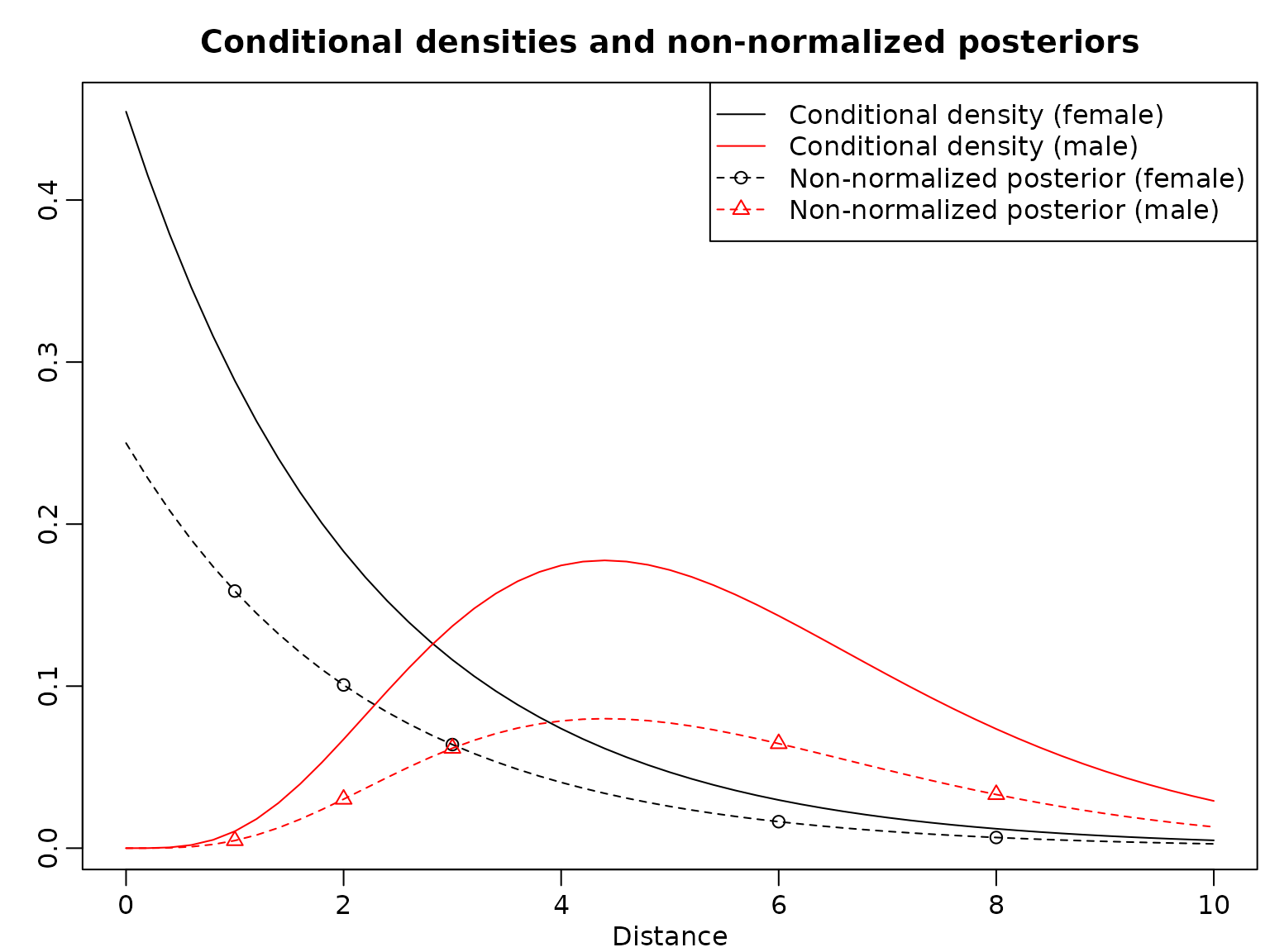

Finally, here are the posterior probabilities. Note that each ratio of the pairs of corresponding posterior probabilities is the same as each ratio of the heights of the vertically corresponding points in the graph.

normalizer <- theta1_y_unnormalized + theta0_y_unnormalized
theta1_y <- theta1_y_unnormalized / normalizer
theta0_y <- theta0_y_unnormalized / normalizer
res <- rbind(female = theta1_y, male = theta0_y)
colnames(res) <- y
knitr::kable(round(res, 3))

	1	2	3	6	8
female	0.971	0.769	0.509	0.202	0.166
male	0.029	0.231	0.491	0.798	0.834

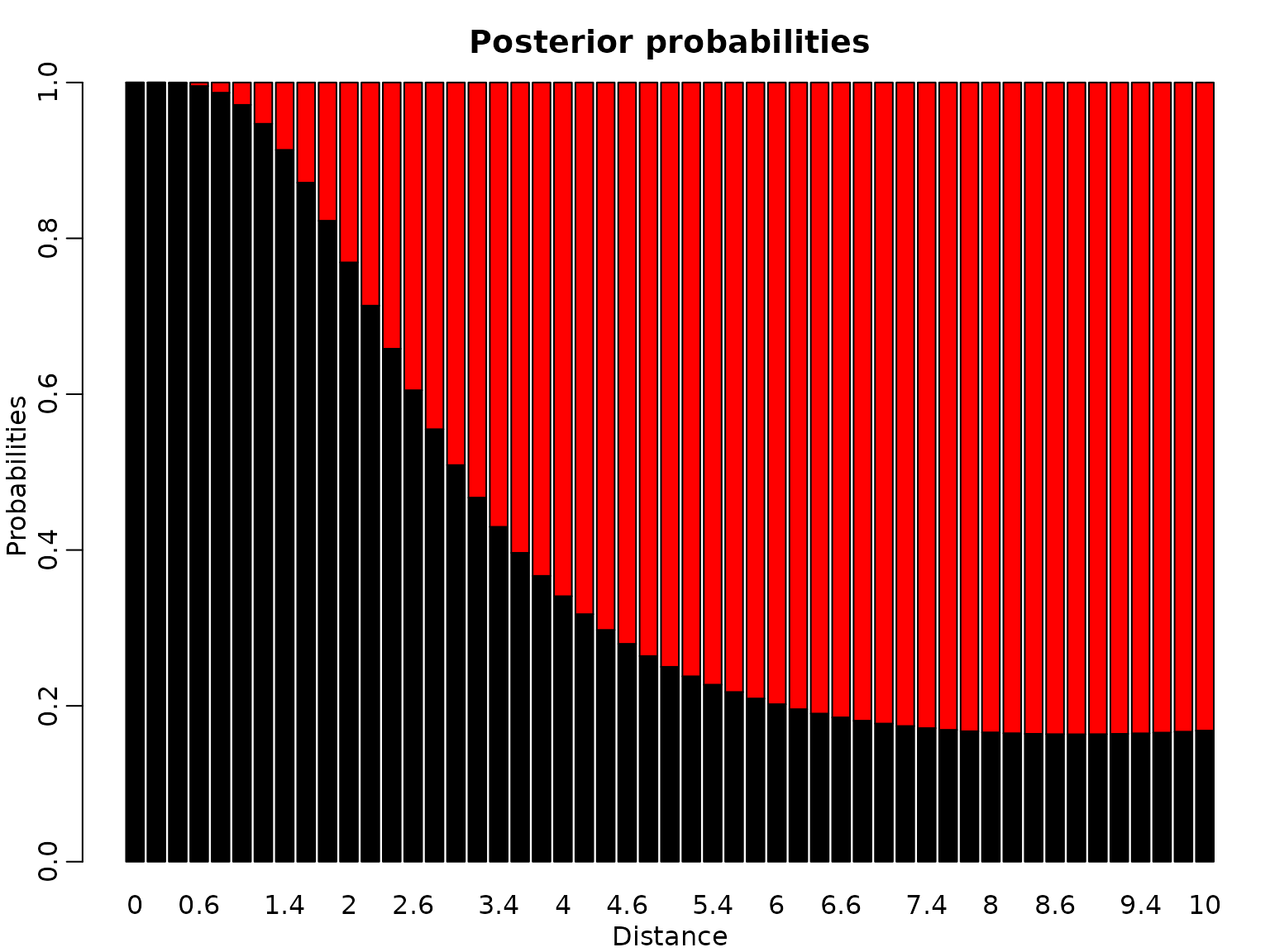
We also plot the posterior probabilities for distance values $y$ ranging from 0 to 10 in steps of 0.2 in a stacked barplot.

normalizer <- theta1_y_all_unnormalized + theta0_y_all_unnormalized
theta1_y_all <- theta1_y_all_unnormalized / normalizer
theta0_y_all <- theta0_y_all_unnormalized / normalizer
res <- rbind(female = theta1_y_all, male = theta0_y_all)
colnames(res) <- y_all
barplot(res, main = "Posterior probabilities", xlab = "Distance",
        ylab = "Probabilities", col = c("black", "red"))