Chapter 2: A First Bayesian Analysis of Count Data • BayesianLearningCode

Section 2.1

Example 2.2: Road Safety Data

Let us first take a look at the data.

data("accidents", package = "BayesianLearningCode")
summary(accidents)
#>  children_accidents children_exposure seniors_accidents seniors_exposure
#>  Min.   :0.000      Min.   :8171      Min.   : 0.00     Min.   :42854   
#>  1st Qu.:1.000      1st Qu.:8678      1st Qu.: 3.00     1st Qu.:43574   
#>  Median :2.000      Median :8900      Median : 5.00     Median :44097   
#>  Mean   :1.839      Mean   :8856      Mean   : 5.25     Mean   :43890   
#>  3rd Qu.:3.000      3rd Qu.:9103      3rd Qu.: 7.00     3rd Qu.:44264   
#>  Max.   :5.000      Max.   :9204      Max.   :15.00     Max.   :44671
plot(accidents[, c("children_accidents", "children_exposure")],
     mar = c(0, 0, 0, 0), oma = c(3, 3, 1.5, .1),
     main = "", xlab = "", ylab = "", ann = FALSE)
title("Road accidents involving pedestrian children", line = 1.7)
mtext(c("Accidents", "Exposure"), side = 2, line = 1.5, adj = c(0.77, 0.29))
mtext("Time", side = 1, line = 1.5, at = 1995.6)


plot(accidents[, c("seniors_accidents", "seniors_exposure")],
     mar = c(0, 0, 0, 0), oma = c(3, 3, 1.5, .1),
     main = "", xlab = "", ylab = "", ann = FALSE)
title("Road accidents involving pedestrian seniors", line = 1.7)
mtext(c("Accidents", "Exposure"), side = 2, line = 1.5, adj = c(0.77, 0.29))
mtext("Time", side = 1, line = 1.5, at = 1995.6)

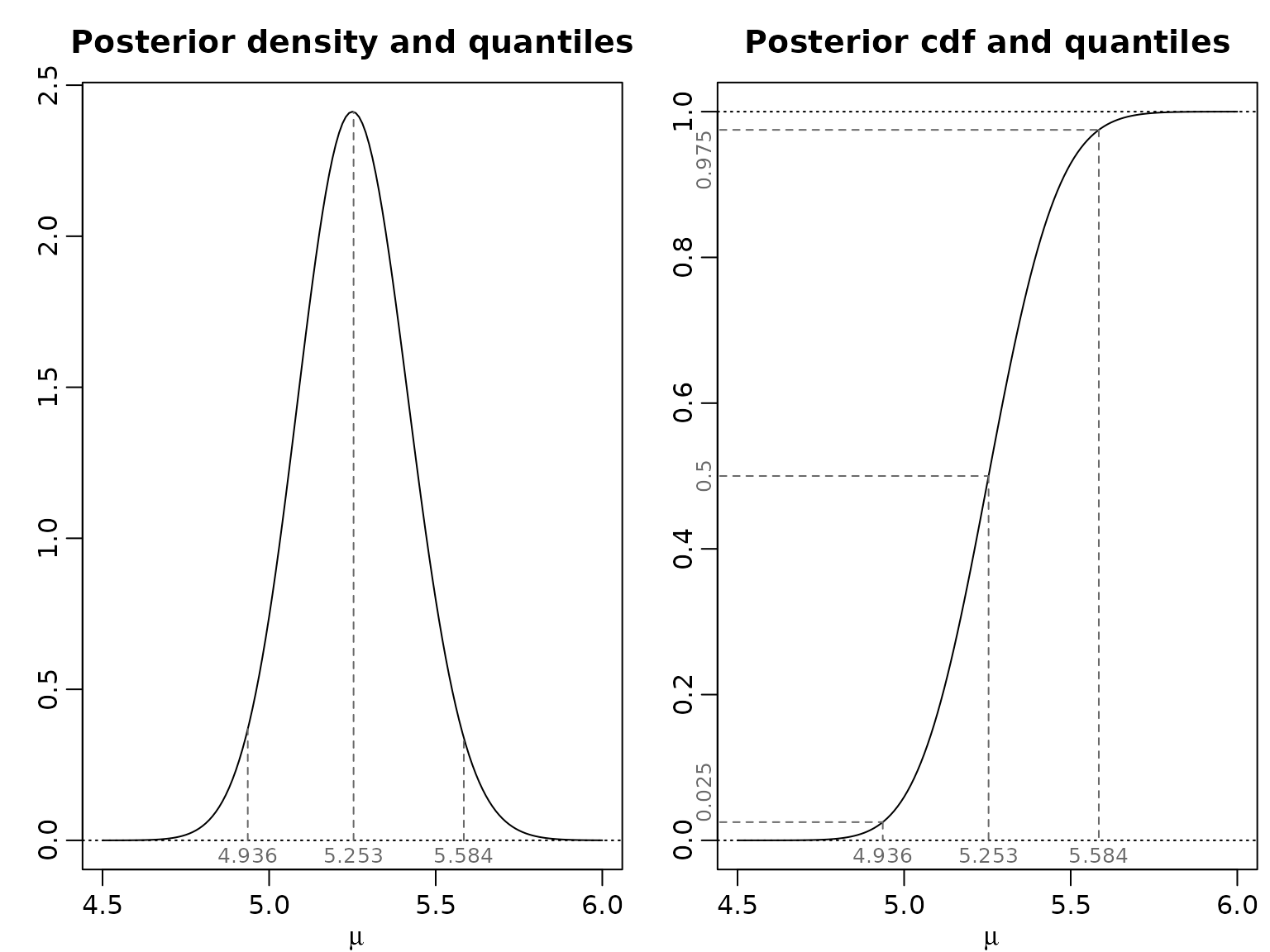
Example 2.3: Posterior inference for the Road Safety Data (flat prior)

The posterior under a flat prior is $\mu|\mathbf{y} \sim \mathcal G(N\bar y + 1, N),$ which we visualize for the seniors, along with the 0.025-, the 0.5-, and the 0.975-quantile.

y <- accidents[, "seniors_accidents"]
aN <- sum(y) + 1
bN <- length(y)

mu <- seq(4.5, 6, by = 0.01)
plot(mu, dgamma(mu, aN, bN), type = "l", xlab = expression(mu), ylab = "",
     main = "Posterior density and quantiles")
abline(h = 0, lty = 3)

probs <- c(0.025, .5, .975)
qs <- qgamma(probs, aN, bN)
round(qs, digits = 3)
#> [1] 4.936 5.253 5.584
ds <- dgamma(qs, aN, bN)

for (i in seq_along(probs)) {
  lines(c(qs[i], qs[i]), c(0, ds[i]), lty = 2, col = "dimgrey")
}
mtext(round(qs, 3), side = 1, at = qs, line = -1, cex = 0.8, col = "dimgrey")

plot(mu, pgamma(mu, aN, bN), type = "l", xlab = expression(mu), ylab = "",
     main = "Posterior cdf and quantiles")
abline(h = c(0, 1), lty = 3)
mtext(round(probs, 3), side = 2, at = probs, adj = c(0, .5, 1), cex = .8, col = "dimgrey")
mtext(round(qs, 3), side = 1, at = qs, line = -1, cex = 0.8, col = "dimgrey")

for (i in seq_along(probs)) {
  lines(c(.9 * min(mu), qs[i]), c(probs[i], probs[i]), lty = 2, col = "dimgrey")
  lines(c(qs[i], qs[i]), c(probs[i], 0), lty = 2, col = "dimgrey")
}

Example 2.4: Posterior inference for the Road Safety Data (gamma prior)

We choose several values for $m_0$ and $a_0$ . Note that, formally, choosing $m_0 = \infty$ and $a_0 = 1$ gives the improper prior from above.

m0 <- c(Inf, mean(y), mean(y), mean(y), 0.5, 3, 10)
a0 <- c(1, 0.5, 2, 10, 3, 3, 3)
plot(mu, dgamma(mu, a0[1] + sum(y), a0[1]/m0[1] + length(y)), type = "l",
     xlab = expression(mu), ylab = "", main = "Posterior density")
for (i in 2:4) {
  lines(mu, dgamma(mu, a0[i] + sum(y), a0[i]/m0[i] + length(y)),
        col = i, lty = i)
}
legend("topright", legend = c(paste0("a0 = ", a0[2:4]), "improper"),
       col = c(2:4, 1), lty = c(2:4, 1))

plot(mu, dgamma(mu, a0[1] + sum(y), a0[1]/m0[1] + length(y)), type = "l",
     xlab = expression(mu), ylab = "", main = "Posterior density")
for (i in 5:7) {
  lines(mu, dgamma(mu, a0[i] + sum(y), a0[i]/m0[i] + length(y)),
        col = i - 3, lty = i - 3)
}
legend("topright", legend = c(paste0("m0 = ", m0[5:7]), "improper"),
       col = c(5:7 - 3, 1), lty = c(5:7 - 3, 1))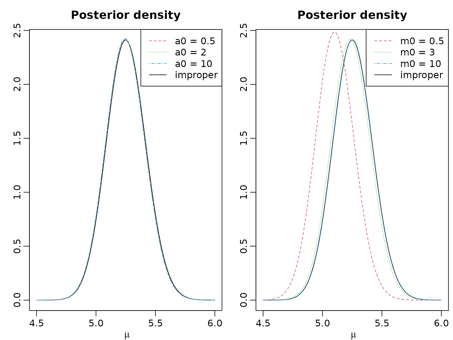

b0 <- a0 / m0
aN <- a0 + sum(y)
bN <- b0 + length(y)
res <- cbind(a0 = a0, b0 = b0, m0 = m0,
             postmean = aN / bN,
             postSD = sqrt(aN / bN^2),
             leftpostquant = qgamma(0.025, aN, bN),
             rightpostquant = qgamma(0.975, aN, bN))
knitr::kable(round(res, 3))

a0	b0	m0	postmean	postSD	leftpostquant	rightpostquant
1.0	0.000	Inf	5.255	0.165	4.936	5.584
0.5	0.095	5.25	5.250	0.165	4.931	5.579
2.0	0.381	5.25	5.250	0.165	4.931	5.579
10.0	1.905	5.25	5.250	0.165	4.932	5.577
3.0	6.000	0.50	5.106	0.161	4.796	5.426
3.0	1.000	3.00	5.238	0.165	4.920	5.566
3.0	0.300	10.00	5.257	0.165	4.938	5.586

Section 2.2

Example 2.8: Including exposures for the Road Safety Data

We now include the exposure at time $i$ , $e_i$ , to estimate the monthly risk $\lambda$ of children to be killed or seriously injured via the following likelihood assumption:

$y_i \sim \mathcal P(\lambda e_i), \quad i = 1,\dots,N.$ Note that we still assume that the data is independently (but not identically!) distributed. We proceed by computing and visualizing the posterior for different prior hyperparameter choices.

y <- accidents[, "children_accidents"]
exp <- accidents[, "children_exposure"]
lambdahat <- mean(y)/mean(exp)
a0 <- c(1, 0.5, 1, 2)
b0 <- c(0, a0[-1]/lambdahat)
aN <- a0 + sum(y)
bN <- b0 + sum(exp)

lambda <- seq(0.00016, 0.00026, by = .000001)
plot(lambda, dgamma(lambda, aN[1], bN[1]), type = "l",
     xlab = expression(lambda), ylab = "",
     main = "Posterior densities for various priors")
for (i in 2:length(aN)) lines(lambda, dgamma(lambda, aN[i], bN[i]), lty = i, col = i)

hyperparams <- paste0("a0 = ", formatC(a0, 1, format = "f"),
                      ", ", "b0 = ", round(b0))

legend("topright", hyperparams, lty = 1:4, col = 1:4)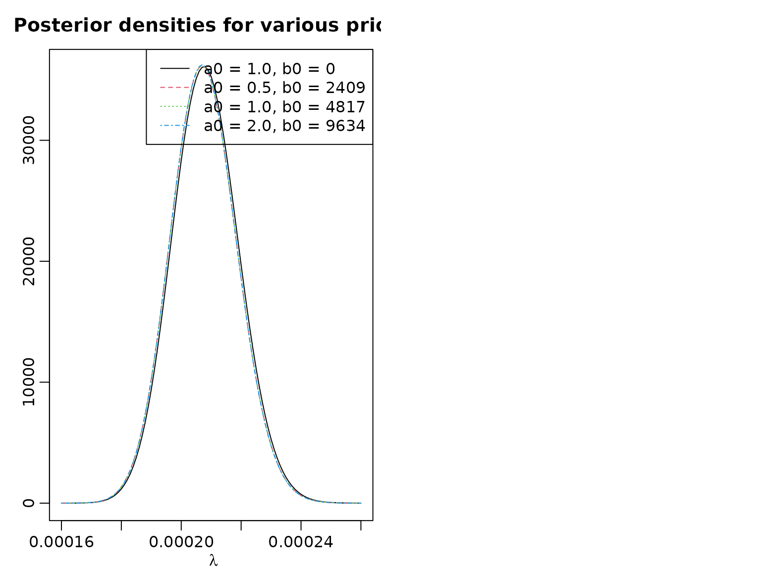

For all our data-driven priors, we get the same posterior mean. The credible intervals differ slightly.

postmean <- aN/bN
leftpostquant <- qgamma(.025, aN, bN)
rightpostquant <- qgamma(.975, aN, bN)
res <- cbind(leftpostquant, postmean, rightpostquant)
rownames(res) <- hyperparams
res
#>                     leftpostquant     postmean rightpostquant
#> a0 = 1.0, b0 = 0     0.0001870605 0.0002081851   0.0002304234
#> a0 = 0.5, b0 = 2409  0.0001865176 0.0002075970   0.0002297886
#> a0 = 1.0, b0 = 4817  0.0001865321 0.0002075970   0.0002297725
#> a0 = 2.0, b0 = 9634  0.0001865610 0.0002075970   0.0002297405

Example 2.9: Including a structural break for the Road Safety Data

We now continue with a Poisson model with a (known) structural break at $i = 94$ (that is, in October 1994). Because the data is stored as a time series (ts) object, we can use the window function to conveniently extract the two time frames.

accidents1 <- window(accidents, end = c(1994, 9))
accidents2 <- window(accidents, start = c(1994, 10))

a01 <- a02 <- 1
b01 <- b02 <- 0

aN1 <- a01 + sum(accidents1[, "children_accidents"])
aN2 <- a02 + sum(accidents2[, "children_accidents"])
bN1 <- b01 + length(accidents1[, "children_accidents"])
bN2 <- b02 + length(accidents2[, "children_accidents"])

post <- function(x1, x2, aN1, aN2, bN1, bN2) {
  dgamma(x1, aN1, bN1) * dgamma(x2, aN2, bN2)
}

mu1 <- seq(1, 3, by = 0.03)
mu2 <- mu1
z <- outer(mu1, mu2, post, aN1 = aN1, aN2 = aN2, bN1 = bN1, bN2 = bN2)

nrz <- nrow(z)
ncz <- ncol(z)

# Generate the desired number of colors from this palette
nbcol <- 20
color <- topo.colors(nbcol)

# Compute the z-value at the facet centres

zfacet <- z[-1, -1] + z[-1, -ncz] + z[-nrz, -1] + z[-nrz, -ncz]
# Recode facet z-values into color indices
facetcol <- cut(zfacet, nbcol)

persp(mu1, mu2, z, col = color[facetcol], ticktype = "detailed", zlab = "",
      xlab = "mu1", ylab = "mu2",
      phi = 20, theta = -30)

contour(mu1, mu2, z, col = color, xlab = bquote(mu[1]), ylab = bquote(mu[2]))
abline(0,1)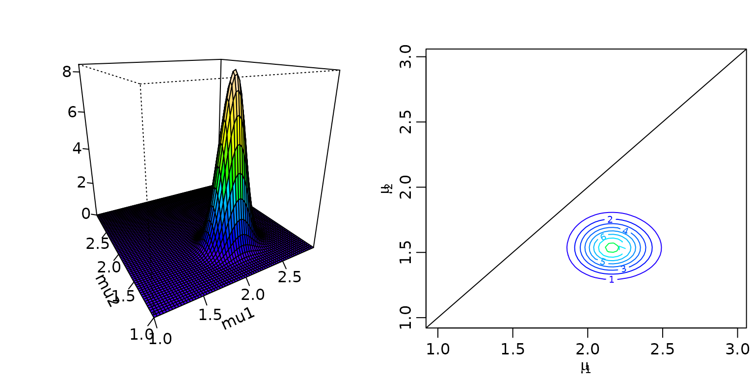

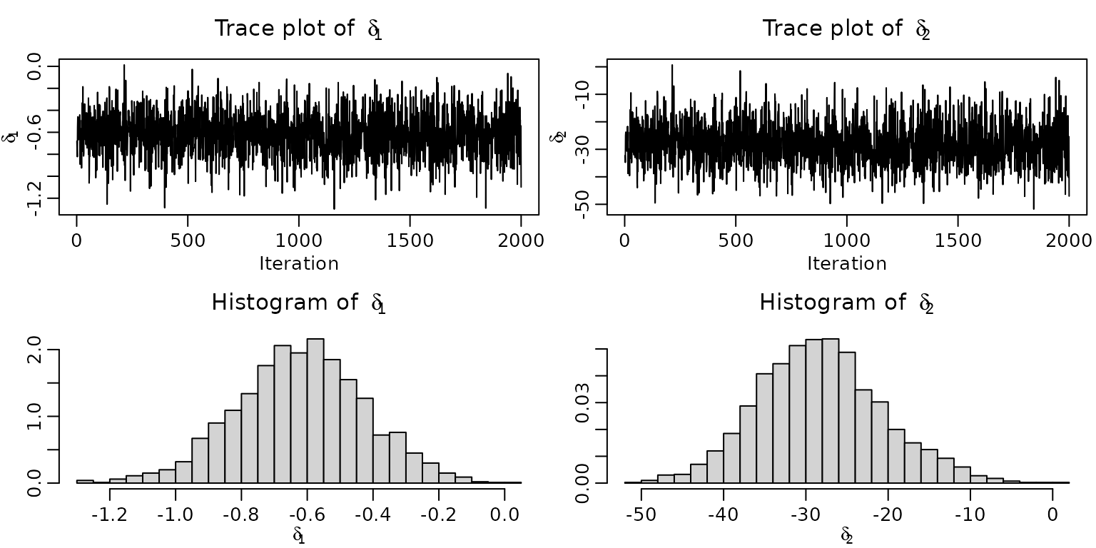
Example 2.10: Obtaining posterior draws for the Road Safety Data

We now proceed with simple Monte Carlo approximation of (nonlinear) functionals of the posterior.

set.seed(1)

nsamp <- 2000
mu1 <- rgamma(nsamp, aN1, bN1)
mu2 <- rgamma(nsamp, aN2, bN2)
delta1 <- mu2 - mu1
delta2 <- 100 * (mu2 - mu1) / mu1


ts.plot(delta1, main = bquote("Trace plot of " ~ delta[1]),
        ylab = expression(delta[1]), xlab = "Iteration")
ts.plot(delta2, main = bquote("Trace plot of " ~ delta[2]),
        ylab = expression(delta[2]), xlab = "Iteration")
hist(delta1, breaks = 20, prob = TRUE, xlab = expression(delta[1]), ylab = "",
     main = bquote("Histogram of " ~ delta[1]))
hist(delta2, breaks = 20, prob = TRUE, xlab = expression(delta[2]), ylab = "",
     main = bquote("Histogram of " ~ delta[2]))