Chapter 3: A First Bayesian Analysis of Unknown Probabilities • BayesianLearningCode

Section 3.1: Data arising from a homogeneous population: The beta-binomial model

Figure 3.1: Posteriors under the beta-binomial model

To reproduce the posteriors in this figure, we simply need to plug in the respective counts into the expression for the posterior density and visualize it accordingly.

trueprop <- c(0, .1, .5)
N <- c(100, 400)
theta <- seq(0, 1, .001)

for (p in trueprop) {
  for (n in N) {
    aN <- n * p + 1
    bN <- n - n * p + 1
    plot(theta, dbeta(theta, aN, bN), type = "l", xlab = expression(vartheta),
         ylab = "", main = bquote(N == .(n) ~ "and" ~ S[N] == .(n * p)))
  }
}

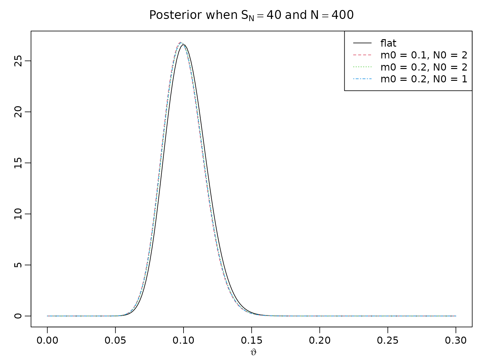
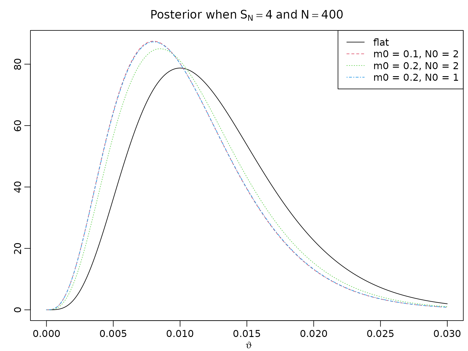
Calibrating the Beta prior

Let $m_0 = \frac{a_0}{a_0 + b_0}$ denote the prior mean and $N_0 = a_0 + b_0$ the strength of the prior information.

m0 <- c(.5, .1, .2, .2)
N0 <- c(2, 2, 2, 1)
a <- N0 * m0
b <- N0 * (1 - m0)
N <- 400
SN <- c(40, 4)

for (i in seq_along(SN)) {
  aN <- SN[i] + a
  bN <- N - SN[i] + b
  theta <- seq(0, 3 * SN[i] / N, length.out = 200)
  plot(theta, dbeta(theta, aN[1], bN[1]), type = "l", ylab = "",
       xlab = expression(vartheta), ylim = range(dbeta(theta, aN, bN)),
       main = bquote("Posterior when" ~ S[N] == .(SN[i]) ~ "and" ~ N == .(N)))
  for (j in 2:4) {
    lines(theta, dbeta(theta, aN[j], bN[j]), col = j, lty = j)
  }
  legend("topright", c("flat", paste(paste0("m0 = ", m0[2:4]),
                                     paste0(" N0 = ", N0[2:4]), sep = ",")),
         lty = 1:4, col = 1:4)
}

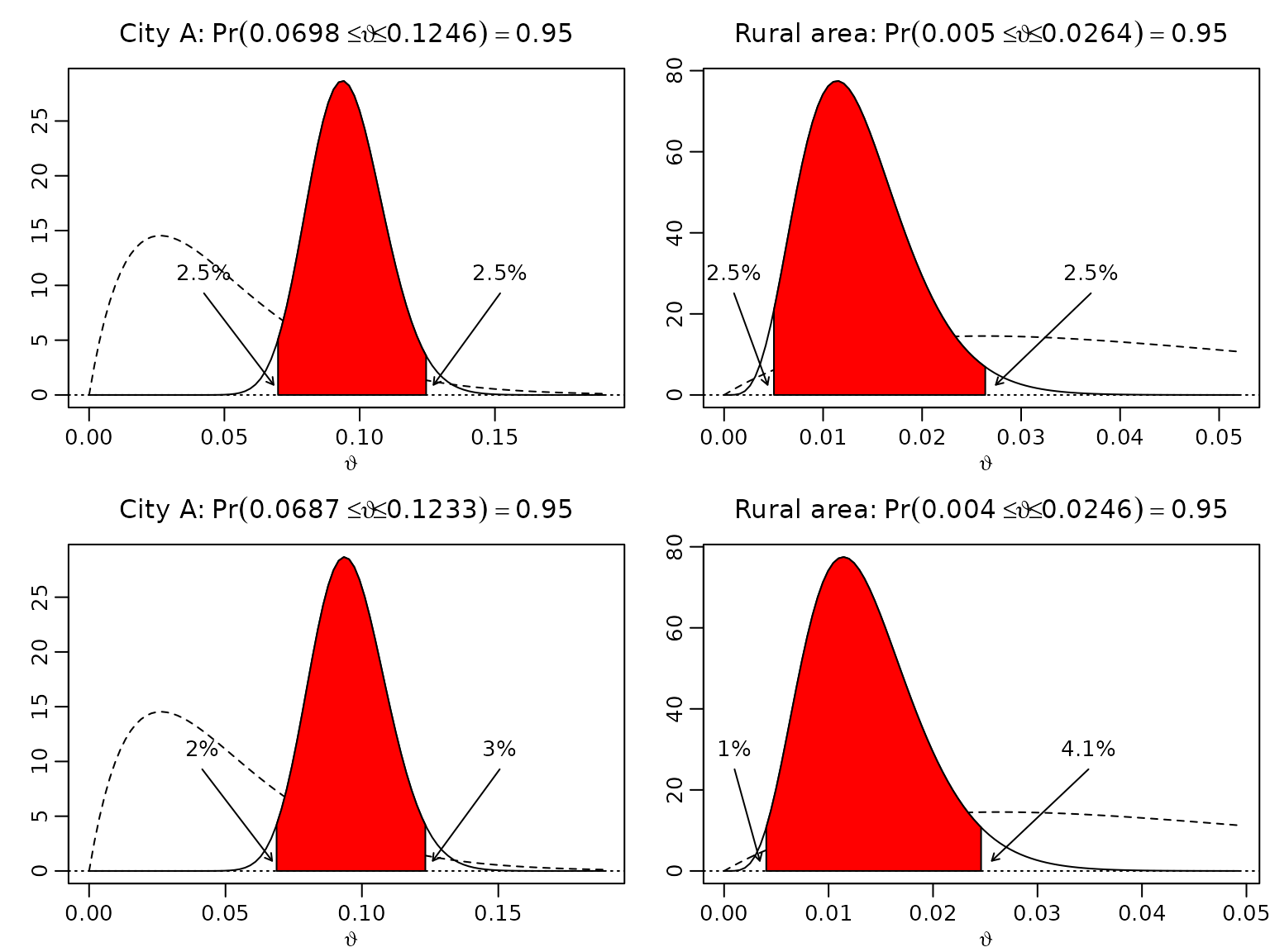
Example 3.1 / Figure 3.2: Uncertainty quantification for market shares

In city A, 40 out of 400 questioned people would purchase a certain product, in a rural community, only 4 out of 400. Assuming a uniform prior, we now compute equal-tailed intervals and highest posterior density (HPD) intervals. Note that R is (generally) vectorized, so we can compute the equal-tailed intervals without using a loop.

m0 <- 0.05
N0 <- 40
a <- N0 * m0
b <- N0 * (1 - m0)
N <- 400
SN <- c("City A" = 40, "Rural area" = 4)
aN <- SN + a
bN <- N - SN + b

gamma <- .95
alpha <- 1 - gamma

# Equal-tailed credible intervals
leftET <- qbeta(alpha/2, aN, bN)
rightET <- qbeta(1 - alpha/2, aN, bN)

# HPD intervals
resolution <- 10000
grid <- seq(0, 1, length.out = resolution + 1)
dist <- gamma * resolution

leftHPD <- rightHPD <- rep(NA_real_, length(aN))
for (i in seq_along(aN)) {
  qs <- qbeta(grid, aN[i], bN[i])
  minimizer <- which.min(diff(qs, lag = dist))
  leftHPD[i] <- qs[minimizer]
  rightHPD[i] <- qs[minimizer + dist]
}

Now we visualize our findings.

left <- cbind(leftET, leftHPD)
right <- cbind(rightET, rightHPD)

for (i in seq_along(aN)) {
  for (j in seq_len(ncol(left))) {
    len <- right[i,j] - left[i,j]
    theta <- seq(0, right[i,j] + 1.2 * len, length.out = 100)
  
    plot(theta, dbeta(theta, aN[i], bN[i]), type = "l",
         xlab = expression(vartheta), ylab = "",
         main = bquote(.(names(aN[i])) * ":" ~ Pr(.(round(left[i,j], 4)) <=
                       {vartheta <= .(round(right[i,j], 4))}) == .(gamma)))
    lines(theta, dbeta(theta, a, b), lty = 2)
    abline(h = 0, lty = 3)
  
    polygon(c(left[i,j], left[i,j],
              theta[theta > left[i,j] & theta < right[i,j]],
              right[i,j], right[i,j]),
            c(0, dbeta(left[i,j], aN[i], bN[i]),
              dbeta(theta[theta >= left[i,j] & theta <= right[i,j]], aN[i], bN[i]),
              dbeta(right[i,j], aN[i], bN[i]), 0),
          col = "red")
    arrows(x0 <- max(left[i,j] - .5 * len, 0.001),
           y0 <- .3 * diff(par("usr")[3:4]),
           x1 <- left[i,j] - .03 * len,
           y1 <- .03 * diff(par("usr")[3:4]),
           length = .05)
    text(x0, y0, paste0(round(100 * pbeta(left[i,j], aN[i], bN[i]), 1), "%"),
         pos = 3)
    
    arrows(x0 <- right[i,j] + .5 * len,
           y0 <- .3 * diff(par("usr")[3:4]),
           x1 <- right[i,j] + .05 * len,
           y1 <- .03 * diff(par("usr")[3:4]),
           length = .05)
    text(x0, y0, paste0(round(100 * (1 - pbeta(right[i,j], aN[i], bN[i])), 1), "%"),
         pos = 3)
  }
}

Example 3.2 / Table 3.1: Posterior credible intervals under the beta-binomial model

We now proceed to computing credible intervals for the synthetic example.

Ns <- rep(N, each = length(trueprop))
SNs <- Ns * rep(trueprop, length(N))

aN <- SNs + 1    
bN <- Ns - SNs + 1
    
# Equal-tails credible intervals
leftET <- qbeta(alpha/2, aN, bN)
rightET <- qbeta(1 - alpha/2, aN, bN)

# HPD intervals
resolution <- 10000
grid <- seq(0, 1, length.out = resolution + 1)
dist <- gamma * resolution

leftHPD <- rightHPD <- rep(NA_real_, length(aN))
for (i in seq_along(aN)) {
  qs <- qbeta(grid, aN[i], bN[i])
  minimizer <- which.min(diff(qs, lag = dist))
  leftHPD[i] <- qs[minimizer]
  rightHPD[i] <- qs[minimizer + dist]
}

res <- cbind(leftET, rightET, leftHPD, rightHPD)

All the desired intervals are now stored and can be displayed.

knitr::kable(round(res, 4))

leftET	rightET	leftHPD	rightHPD
0.0001	0.0092	0.0000	0.0074
0.0744	0.1334	0.0732	0.1319
0.4512	0.5488	0.4512	0.5488

We can also compare their lengths.

res <- cbind(lengthET = rightET - leftET, lengthHPD = rightHPD - leftHPD)
knitr::kable(round(res, 4))

lengthET	lengthHPD
0.0091	0.0074
0.0590	0.0587
0.0976	0.0976

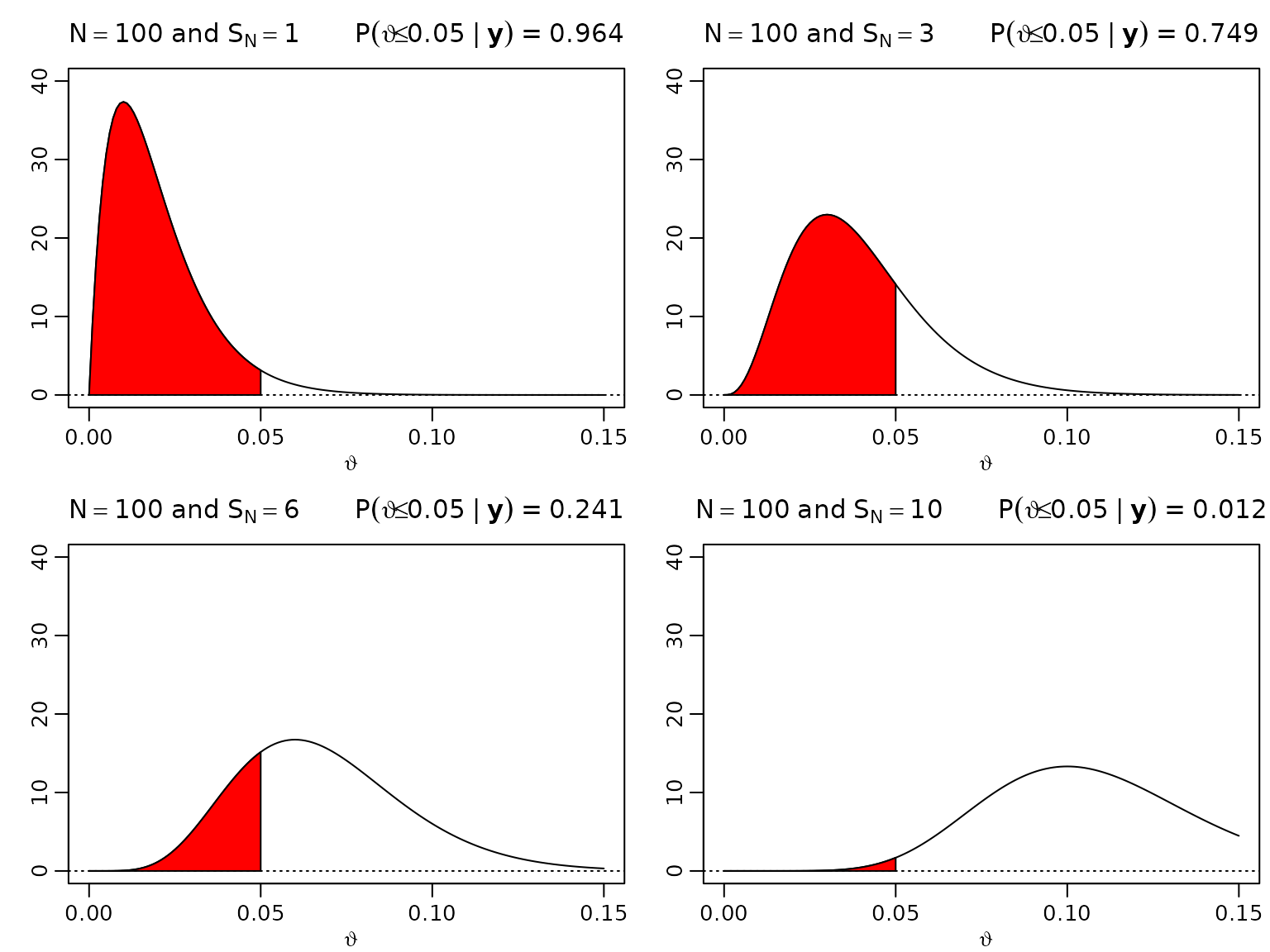
Figure 3.3: One-sided hypothesis testing

We now move forward to assessing visualizing the posterior probability of $\vartheta$ (the proportion of defective items) being less than $1/20 = 0.05$ for $N = 100$ and $S_N \in \{1,3,6,10\}$ .

theta <- seq(0, .15, .001)
N <- 100
SN <- c(1, 3, 6, 10)
aN <- SN + 1
bN <- N - SN + 1
for (i in seq_along(SN)) {
  plot(theta, dbeta(theta, aN[i], bN[i]), type = "l", ylim = c(0, 40),
       xlab = expression(vartheta), ylab = "",
       main = bquote(N == 100 ~ "and" ~ S[N] == .(SN[i]) ~ "     " ~
                       P(vartheta <= 0.05 ~ "|" ~ bold(y)) ~ "=" ~
                       .(round(pbeta(0.05, aN[i], bN[i]), 3))))
  abline(h = 0, lty = 3)
  polygon(c(theta[theta <= 0.05], 0.05),
          c(dbeta(theta[theta <= 0.05], aN[i], bN[i]), 0), col = "red")
}

Example 3.4: Labor market data

We load the dataset from the package and extract the data needed for the anlaysis:

data("labor", package = "BayesianLearningCode")
labor <- subset(labor,
                income_1997 != "zero" & female,
                c(income_1998, wcollar_1986))
labor <- with(labor,
              data.frame(unemployed = income_1998 == "zero",
                         wcollar = wcollar_1986))

Cross-tabuling being unemployed (i.e., having no income) and being a white collar work gives:

table(labor)
#>           wcollar
#> unemployed FALSE TRUE
#>      FALSE   368  634
#>      TRUE     62   59

We estimate the risk for a woman who had a positive income, to have no income in the next year and assume that this risk is different for white- and blue-collar workers.

The four relevant data summaries are given by:

(N1 <- with(labor, sum(wcollar)))
#> [1] 693
(S_N1 <- with(labor, sum(wcollar & unemployed)))
#> [1] 59
(N2 <- with(labor, sum(!wcollar)))
#> [1] 430
(S_N2 <- with(labor, sum(!wcollar & unemployed)))
#> [1] 62

Under a uniform prior, the parameters of the posterior distribution are given by:

aN1 <- 1 + S_N1
bN1 <- 1 + N1 - S_N1
aN2 <- 1 + S_N2
bN2 <- 1 + N2 - S_N2

The posterior expectations are given by

aN1 / (aN1 + bN1)
#> [1] 0.08633094
aN2 / (aN2 + bN2)
#> [1] 0.1458333

We visualize the joint posterior of $(\vartheta_1, \vartheta_2)$ using a contour plot as well as a density estimate of the difference $\vartheta_1 - \vartheta_2$ .

if (pdfplots) {
  pdf("3-2_1.pdf", width = 8, height = 5)
  par(mgp = c(1, .5, 0), mar = c(2.2, 1.5, 2, .2), lwd = 2)
}
par(mfrow = c(1, 2))
post <- function(x1, x2, aN1, aN2, bN1, bN2) {
  dbeta(x1, aN1, bN1) * dbeta(x2, aN2, bN2)
}

vartheta1 <- seq(0.04, 0.13, length.out = 100)
vartheta2 <- seq(0.08, 0.22, length.out = 100)
z <- outer(vartheta1, vartheta2, post, aN1 = aN1, aN2 = aN2, bN1 = bN1, bN2 = bN2)

nrz <- nrow(z)
ncz <- ncol(z)

# Generate the desired number of colors from this palette
nbcol <- 20
color <- topo.colors(nbcol)

# Compute the z-value at the facet centres

zfacet <- z[-1, -1] + z[-1, -ncz] + z[-nrz, -1] + z[-nrz, -ncz]
# Recode facet z-values into color indices
facetcol <- cut(zfacet, nbcol)

contour(vartheta1, vartheta2, z, col = color,
        xlab = bquote(vartheta[1]), ylab = bquote(vartheta[2]),
        main = expression(paste("Posterior of (", vartheta[1],
                                ", ", vartheta[2], ")")))
abline(0,1)
postdraws <- data.frame(vartheta1 = rbeta(10^6, aN1, bN1),
                        vartheta2 = rbeta(10^6, aN2, bN2))
postdraws$diff <- with(postdraws, vartheta2 - vartheta1)
plot(density(postdraws$diff),
     xlab = bquote(vartheta[1] - vartheta[2]),
     main = expression(paste("Posterior density p(", vartheta[1],
                                " - ", vartheta[2], "| y)")))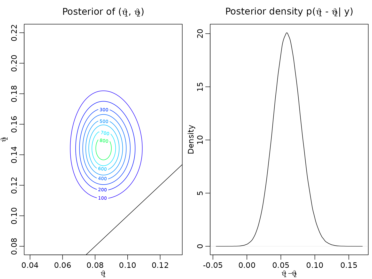

if (pdfplots) {
  pdf("3-2_1.pdf", width = 8, height = 5)
  par(mgp = c(1, .5, 0), mar = c(2.2, 1.5, 2, .2), lwd = 2)
}
par(mfrow = c(1, 3))
labels <- c(bquote(vartheta[1]),
            bquote(vartheta[2]),
            bquote(vartheta[2] - vartheta[1]))
for (i in 1:3) {
    plot(postdraws[1:1000, i], type = "l", ylim = c(0, 0.25),
         xlab = "draw", ylab = labels[i])
}

Example 3.5: Bag of words

Preparing the data

After reading in the quote, we do some simple manipulation such as converting to lower case, getting rid of newlines, and splitting the string into individual words. Finally, we remove potential empty words and display the resulting frequencies.

string <- "You can fool some of the people all of the time,
and all of the people some of the time,
but you can not fool all of the people all of the time."

tmp <- tolower(string)                  ## convert to lower case
tmp <- gsub("\n", " ", tmp)             ## replace newlines with spaces
tmp <- unlist(strsplit(tmp, " |,|\\.")) ## split at spaces, commas, or stops
dat <- tmp[tmp != ""]                   ## remove empty words
tab <- table(dat)
knitr::kable(t(tab))

all	and	but	can	fool	not	of	people	some	the	time	you
4	1	1	2	2	1	6	3	2	6	3	2

To define our universe of possible words, we first look at the words dataset (shipped with this package). It contains 1000 most common English words, alongside their frequency of usage among a total of 100 million occurrences (cf. https://www.eapfoundation.com/vocab/general/bnccoca/).

data("words", package = "BayesianLearningCode")
head(words)
#>       word frequency
#> 1        a   2525253
#> 2     able     47760
#> 3    about    192168
#> 4    above     25370
#> 5 absolute      9284
#> 6   accept     29026

For illustration purposes, we only use the top 50 words and augment those with a question mark for all other words. This leaves us with 51 possible outcomes (our universe).

top50 <- tail(words[order(words$frequency),], 50)
universe <- c("?", sort(top50$word))
freq <- c(10^8 - sum(top50$frequency), top50$frequency[order(top50$word)])
universe
#>  [1] "?"     "a"     "all"   "and"   "as"    "at"    "be"    "but"   "by"   
#> [10] "can"   "do"    "for"   "from"  "get"   "go"    "have"  "he"    "i"    
#> [19] "if"    "in"    "it"    "make"  "more"  "no"    "not"   "of"    "on"   
#> [28] "one"   "or"    "out"   "say"   "she"   "so"    "some"  "that"  "the"  
#> [37] "there" "they"  "this"  "time"  "to"    "up"    "we"    "what"  "when" 
#> [46] "which" "who"   "will"  "with"  "would" "you"

Now, we check if there are any words in our data set which are not included in our universe (here, only fool and people) and replace these with a question mark.

dat[!(dat %in% universe)] <- "?"
knitr::kable(t(table(dat)))

?	all	and	but	can	not	of	some	the	time	you
5	4	1	1	2	1	6	2	6	3	2

Computing the posterior under the uniform prior

Under a uniform prior (i.e., all 51 elements of our universe receive one pseudo-count), the posterior mean for each word occurrence probability is given by $E(\eta_k|\boldsymbol{y}) = \frac{1+N_k}{ 51 + N}, \quad k=1,\ldots,51,$ where $N_k$ stands for the number of data occurrences of the $k$ th word in the universe, and $N$ is the sum of all $N_k$ s. This can be very easily implemented by merging the universe and the data, and simply counting the resulting frequencies.

merged <- c(universe, dat)
counts <- table(merged) - 1L
post_uniform_unnormalized <- 1 + counts
post_uniform <- post_uniform_unnormalized / sum(post_uniform_unnormalized)

Computing the posterior under a less informative indifference prior

Note that the above strategy implicitly assumes that we have exactly 51 pseudo-observations. To render the prior less influential, we can rescale it to, e.g., 1 pseudo-observation. Then, the posterior expectation is $E(\eta_k|\boldsymbol{y}) = \frac{1/51+N_k}{1 + N}, \quad k=1,\ldots,51.$ To compute this expectation we simply add counts and the new pseudo-counts $\gamma_{0,1}, = \gamma_{0,2} = \dots = \gamma_{0,K} = 1/K$ .

K <- length(universe)
N0 <- 1
gamma0 <- rep(N0 / K, length(universe))
post_lessinformative_unnormalized <-  gamma0 + counts
post_lessinformative <-
  post_lessinformative_unnormalized / sum(post_lessinformative_unnormalized)

Alternatively, we could use a loop.

post_lessinformative_unnormalized2 <- rep(NA_real_, length(universe))
for (i in seq_along(universe)) {
  Nk <- sum(dat == universe[i])
  post_lessinformative_unnormalized2[i] <- gamma0[i] + Nk
}
post_lessinformative2 <-
  post_lessinformative_unnormalized2 / sum(post_lessinformative_unnormalized2)

The results must be numerically equivalent, and we can verify this easily.

all(abs(post_lessinformative - post_lessinformative2) < 1e-10)
#> [1] TRUE

Summing up what we have so far.

dirichlet_sd <- function(gamma) {
  mean <- gamma / sum(gamma)
  sd <- sqrt((mean * (1 - mean)) / (sum(gamma) + 1))
  sd
}

resfull <- cbind(prior_mean = rep(1/K, K),
                 prior_sd_uniform = dirichlet_sd(rep(1, K)),
                 prior_sd_lessinformative = dirichlet_sd(rep(1/K, K)),
                 rel_freq = counts / sum(counts),
                 posterior_mean_uniform = post_uniform,
                 posterior_sd_uniform = dirichlet_sd(post_uniform),
                 posterior_mean_lessinformative = post_lessinformative,
                 posterior_sd_lessinformative = dirichlet_sd(post_lessinformative))

unseen <- counts == 0L
res <- rbind(resfull[!unseen,], UNSEEN = resfull[which(unseen)[1],])
knitr::kable(t(round(res, 4)))

	?	all	and	but	can	not	of	some	the	time	you	UNSEEN
prior_mean	0.0196	0.0196	0.0196	0.0196	0.0196	0.0196	0.0196	0.0196	0.0196	0.0196	0.0196	0.0196
prior_sd_uniform	0.0192	0.0192	0.0192	0.0192	0.0192	0.0192	0.0192	0.0192	0.0192	0.0192	0.0192	0.0192
prior_sd_lessinformative	0.0980	0.0980	0.0980	0.0980	0.0980	0.0980	0.0980	0.0980	0.0980	0.0980	0.0980	0.0980
rel_freq	0.1515	0.1212	0.0303	0.0303	0.0606	0.0303	0.1818	0.0606	0.1818	0.0909	0.0606	0.0000
posterior_mean_uniform	0.0714	0.0595	0.0238	0.0238	0.0357	0.0238	0.0833	0.0357	0.0833	0.0476	0.0357	0.0119
posterior_sd_uniform	0.1821	0.1673	0.1078	0.1078	0.1312	0.1078	0.1954	0.1312	0.1954	0.1506	0.1312	0.0767
posterior_mean_lessinformative	0.1476	0.1182	0.0300	0.0300	0.0594	0.0300	0.1770	0.0594	0.1770	0.0888	0.0594	0.0006
posterior_sd_lessinformative	0.2508	0.2283	0.1206	0.1206	0.1671	0.1206	0.2699	0.1671	0.2699	0.2012	0.1671	0.0170

Computing the posterior under an informed prior

One might consider using yet another prior (which we label informed). For instance, we might want to fix the total number of pseudo-counts $N_0$ to, say, one fifth of the number of observations $N$ (this implies a data to prior ratio of 5 to 1). Each word in the universe is then weighted according to its frequency of appearance in the English language. Remember that the prior probability for a word outside of the top 50 English words is $10^8$ (the total number of words in the corpus) minus the sum of the top 50 counts. To compute the posterior, we can again add the actual counts and the new pseudo-counts.

N <- length(dat)
N0 <- N/5
gamma0 <- N0 * freq / 10^8

post_informed_unnormalized <- gamma0 + counts
post_informed <- post_informed_unnormalized / sum(post_informed_unnormalized)

Alternatively, we might want to prefer heavier shrinkage with respect to the base rate (here, the overall word distribution in the English language). This can simply be accomplished by increasing the total number of pseudo-counts $N_0$ .

N0 <- 5*N
gamma0 <- N0 * freq / 10^8

post_informed_unnormalized2 <- counts + gamma0
post_informed2 <- post_informed_unnormalized2 / sum(post_informed_unnormalized2)

Visualizing the results

To display the results, we use bar plots. We also add the prior probabilities of each word via green triangles and the observed relative frequencies via red circles. Sorting is done via frequency counts.

ord <- order(counts, decreasing = TRUE)
midpts <- barplot(post_uniform[ord], las = 2,
                  ylim = c(0, max(counts/N, post_uniform)))
points(midpts, counts[ord]/N, col = 2, pch = 1)
points(midpts, rep(1/51, length(midpts)), col = 3, pch = 2)
title("Indifference prior (uniform)")
legend("topright", c("Observed frequencies", "Prior expectations"),
       col = 2:3, pch = 1:2)

midpts <- barplot(post_lessinformative[ord], las = 2,
                  ylim = c(0, max(counts/N, post_lessinformative)))
points(midpts, counts[ord]/N, col = 2, pch = 1)
points(midpts, rep(1/51, length(midpts)), col = 3, pch = 2)
title("Indifference prior (light shrinkage)")

midpts <- barplot(post_informed[ord], las = 2,
                   ylim = c(0, max(counts/N, post_informed, freq/10^8)))
points(midpts, counts[ord]/N, col = 2, pch = 1)
points(midpts, freq[ord] / 10^8, col = 3, pch = 2)
title("Informed prior (light shrinkage)")

midpts <- barplot(post_informed2[ord], las = 2,
                   ylim = c(0, max(counts/N, post_informed2, freq/10^8)))
points(midpts, counts[ord]/N, col = 2, pch = 1)
points(midpts, freq[ord] /10^8, col = 3, pch = 2)
title("Informed prior (heavy shrinkage)")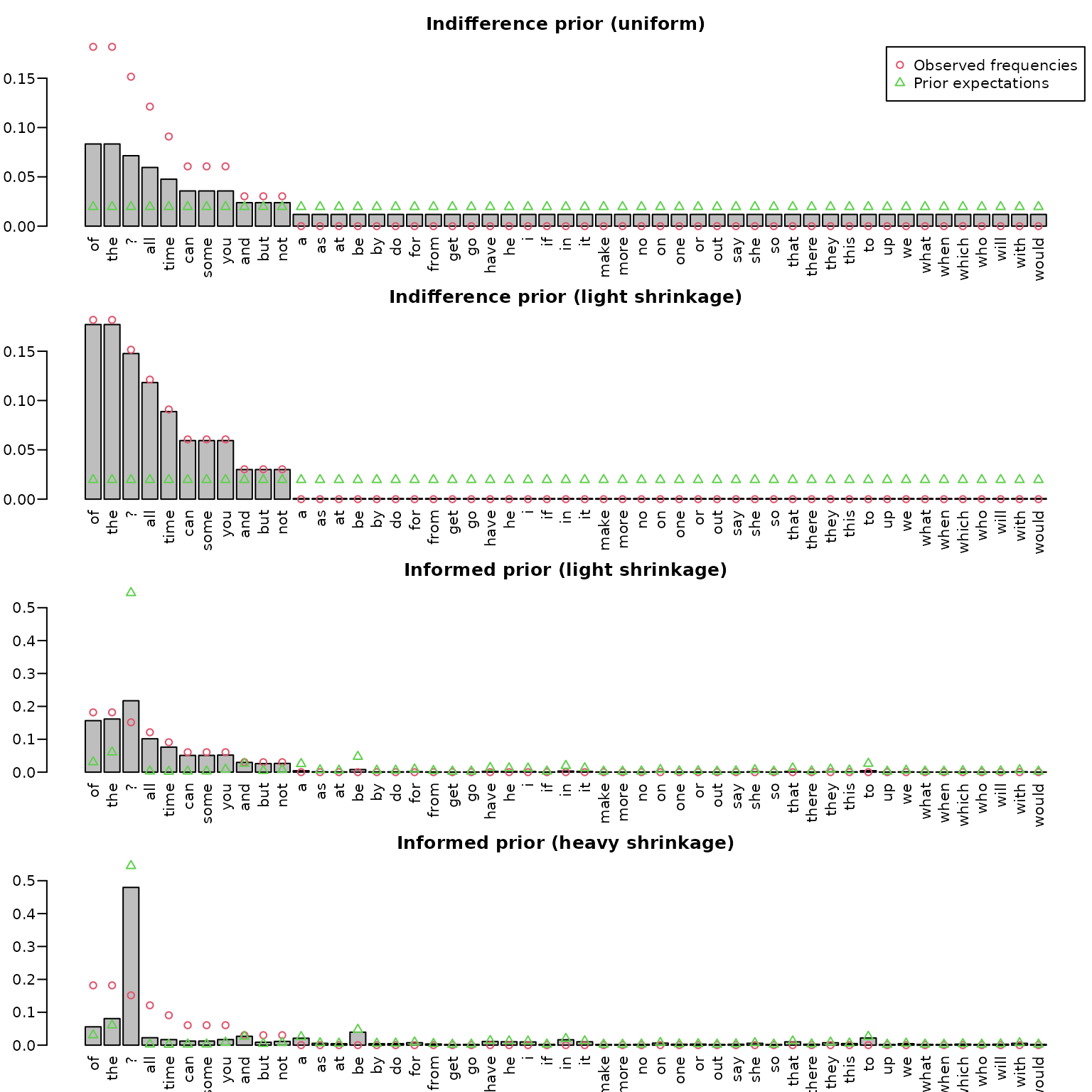

In the top panel (based on the uniform prior), we can nicely see the add-one smoothing effect, i.e., strong shrinkage towards the uniform prior, whereas the second panel shows almost no smoothing/shrinkage, and unseen words are estimated to be extremely unlikely. The two bottom panels show the posteriors under the informed priors, one with light and one with heavy shrinkage towards the prior.