Chapter 8: Beyond Standard Regression Analysis
Chapter08.RmdSection 8.1: Binary response variables
Section 8.1.1: Probit model
Figure 8.1: Latent utility and outcome in the probit model
We start by visualizing a latent utility for a linear predictor with a value of 1.
curve(dnorm(x, mean = 1), from = -3, to = 5, col = "blue",
      xlab = expression(z[i]), ylab = "")
abline(v = 0, col = "red")

dens <- curve(dnorm(x, mean = 1), from = -3, to = 5, n = 161, col = "blue",
              xlab = expression(paste(z[i], "|", y[i], "=0")), ylab = "")
abline(v = 0, col = "red")
polygon(c(dens$x[dens$x <= 0], 0), c(dens$y[dens$x <= 0], 0),
        col = "red", border = NA)

dens <- curve(dnorm(x, mean = 1), from = -3, to = 5, n = 161, col = "blue",
              xlab = expression(paste(z[i], "|", y[i], "=1")), ylab = "" )
abline(v = 0, col = "red")
polygon(c(dens$x[dens$x >= 0], 0), c(dens$y[dens$x >= 0], 0),
        col = "red", border = NA)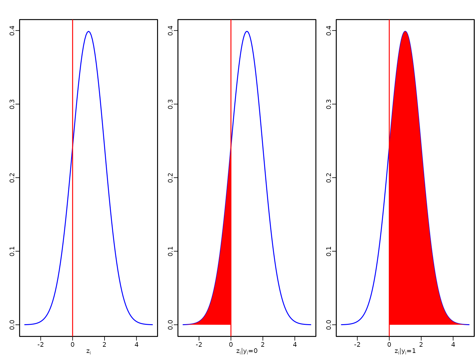
Example 8.1: Labor market data
We now perform probit regression analysis for the labor market data.
library("BayesianLearningCode")
data("labor", package = "BayesianLearningCode")
We model the income in 1998, binarized into unemployed (zero income) and employed, as dependent variable, and use as covariates the variables female (binary), age18 (quantitative, centered at 18 years), wcollar (binary), and unemployed in 1997 (binary). The baseline person is hence an 18 year old male blue collar worker who was employed in 1997.
Example 8.2: Fitting a probit model to the labor market data
The regression coefficients are estimated using data augmentation and Gibbs sampling. We define a function yielding posterior draws using the algorithm detailed in Section 8.1.1.
probit <- function(y, X, b0 = 0, B0 = 10000,
                   burnin = 1000L, M = 20000L / mcmcspeedup) {
  N <- length(y)
  d <- ncol(X) # number of regression effects

  b0 <- rep(b0, length.out = d)
  B0.inv <- diag(rep(1 / B0, length.out = d), nrow = d)
  B0inv.b0 <- B0.inv %*% b0

  betas <- matrix(NA_real_, nrow = M, ncol = d)
  colnames(betas) <- colnames(X)

  z <- rep(NA_real_, N)

  # Define quantities for the Gibbs sampler
  BN <- solve(B0.inv + crossprod(X))
  ind0 <- (y == 0) # indicators for zeros
  ind1 <- (y == 1) # indicators for ones

  # Set starting values
  beta <- c(qnorm(mean(y)), rep(0, d-1))

  for (m in seq_len(burnin + M)) {
    # Draw z conditional on y and beta
    u <- runif(N)
    eta <- X %*% beta
    pi <- pnorm(eta)

    z[ind0] <- eta[ind0] + qnorm(u[ind0] * (1 - pi[ind0]))
    z[ind1] <- eta[ind1] + qnorm(1 - u[ind1] * pi[ind1])

    # Sample beta from the full conditional
    bN <- BN %*% (B0inv.b0 + crossprod(X, z))
    beta <- t(mvtnorm::rmvnorm(1, mean = bN, sigma = BN))

    # Store the beta draws
    if (m > burnin) {
      betas[m - burnin, ] <- beta
    }
 }
 return(betas)
}
We specify the prior on the regression effects as a rather flat normal independence prior and estimate the model parameters.
set.seed(1234)
M <- 20000 / mcmcspeedup
betas <- probit(y_unemp, X_unemp, b0 = 0, B0 = 1000L, burnin = 1000, M = M)
To compute summary statistics from the posterior we use the following function.
res.mcmc <- function(x, lower = 0.025, upper = 0.975) {
  res <- c(quantile(x, lower), mean(x), quantile(x, upper))
  names(res) <- c(paste0(lower * 100, "%"), "Posterior mean",
                  paste0(upper * 100, "%"))
  res
}
We show posterior means and equal-tailed 95% credible intervals of the regression effects.
| 2.5% | Posterior mean | 97.5% | |
|---|---|---|---|
| intercept | -2.123 | -1.968 | -1.824 |
| female | 0.116 | 0.215 | 0.325 |
| age18 | 0.023 | 0.027 | 0.032 |
| wcollar | -0.277 | -0.178 | -0.075 |
| unemp97 | 2.412 | 2.518 | 2.630 |
Next, we determine the estimated risk of unemployment for a baseline person, i.e., a 18 year old male blue collar worker who was employed in 1997, using the posterior mean estimate of the intercept.
The estimated risk to be unemployed in 1998 for a baseline person is very low with a value of 0.0245 and even lower for a white collar worker. This risk is higher for a female, an older person and particularly high if the person was unemployed in 1997.
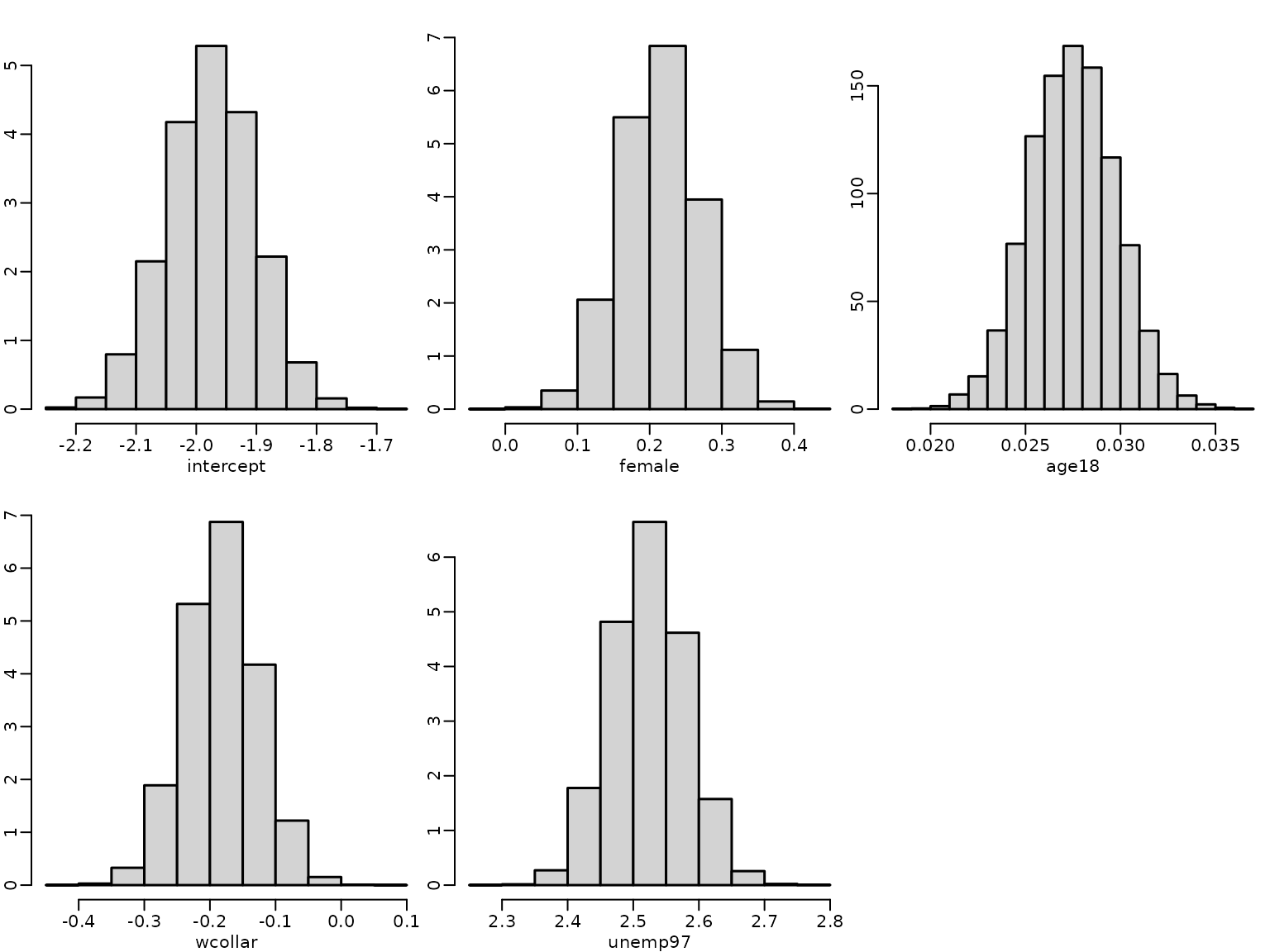
Next, we visualize the estimated posterior distributions for the regression effects by histograms.
for (j in seq_len(ncol(betas))) {
  hist(betas[, j], freq = FALSE, main = "", xlab = colnames(betas)[j],
       ylab = "")
}
A plot of the autocorrelation of the draws shows that although there is some autocorrelation, it vanishes after a few lags.
for (j in seq_len(ncol(betas))) {
    acf(betas[, j], main = "", xlab = "Lag",
        ylab = "empirical ACF")
    title(colnames(betas)[j])
}
We also determine the estimated effective sample sizes (ESSs) to assess the efficiency of the sampler.
ESS <- coda::effectiveSize(betas)
IF <- M / ESS
res_eff <- cbind(ESS = round(ESS, digits = 1),
                 IF = round(IF, digits = 2))
knitr::kable(res_eff)| ESS | IF | |
|---|---|---|
| intercept | 285.4 | 7.01 |
| female | 445.1 | 4.49 |
| age18 | 343.5 | 5.82 |
| wcollar | 400.9 | 4.99 |
| unemp97 | 399.1 | 5.01 |
The estimated effective sample size is at least 285.4 for every regression effect, and hence all estimated inefficiency factors (IFs) are below 7.01.
The sampler is easy to implement, however there might be problems when the response variable contains either only very few or very many successes.
Example 8.3: Imbalanced data
To illustrate this issue, we use data where in trials only 1 failure or only 1 success is observed.
set.seed(1234)

N <- 500
X <- matrix(1, nrow = N)

y1 <- c(0, rep(1, N-1))
betas1 <- probit(y1, X, b0 = 0, B0 = 10000, burnin = 1000, M = M)

y2 <- c(rep(0, N-1), 1)
betas2 <- probit(y2, X, b0 = 0, B0 = 10000, burnin = 1000, M = M)
In both cases the empirical autocorrelation of the draws decreases very slowly and remains high even for a lag of 40.
labels <- expression(beta[0])
plot(betas1, type = "l", main = "N=500, 1 failure", xlab = "Draws after burnin",
     ylab = labels)
acf(betas1, ylab = "empirical ACF")

(ESS1 <- coda::effectiveSize(betas1))
#>     var1
#> 13.77587
(IF1 <- round(M/ESS1, 2))
#>   var1
#> 145.18

plot(betas2, type = "l", main = "N=500, 1 success", xlab = "Draws after burnin",
     ylab = labels)
acf(betas2, ylab = "empirical ACF")
(ESS2 <- coda::effectiveSize(betas2))
#>     var1
#> 29.23532
(IF2 <- round(M/ESS2, 2))
#>  var1
#> 68.41
Hence for these data sets the estimated ESS of the intercept has a value of at most 30, yielding an estimated IF of at most 146.
High autocorrelation in MCMC draws for probit models occurs not only when either successes or failures are rare, but also when a covariate (or a linear combination of covariates) perfectly allows to predict successes and/or failures. Complete separation means that both successes and failures can be perfectly predicted by a covariate, whereas quasi-complete separation means that only either successes or failures can be predicted perfectly.
Example 8.4: Complete separation
To illustrate the effect of complete separation on the estimates, we generate observations where half of them are successes and the other half are failures. We add a binary predictor where for we observe only successes and for only failures.
N <- 500
ns <- 250
x_sep <- rep(c(0, 1), c(ns, N - ns))
y <- rep(c(0, 1), c(ns, N - ns))

table(x_sep, y)
#>      y
#> x_sep   0   1
#>     0 250   0
#>     1   0 250
We estimate the model parameters under the Normal prior with mean and variance matrix and run the sampler for iterations after a burn-in of 1000.
From the plot of the empirical ACF of the draws we see that autocorrelations are close to 1 even at lag 40.
set.seed(1234)
X_sep <- cbind(rep(1, N), x_sep)
betas_sep <- probit(y, X_sep, b0 = 0, B0 = 10000, burnin = 1000, M = M)

labels <- expression(beta[0], beta[1])
plot(betas_sep[, 1], type = "l", xlab = "Draws after burn-in", ylab = labels[1])
acf(betas_sep[, 1], ylab = "empirical ACF")

plot(betas_sep[, 2], type = "l", xlab = "Draws after burn-in", ylab = labels[2])
acf(betas_sep[, 2], ylab = "empirical ACF")
(ESS_sep <- coda::effectiveSize(betas_sep))
#>             x_sep
#> 6.132027 3.458701
(IF_sep <- M/ESS_sep)
#>             x_sep
#> 326.1564 578.2518
Hence the estimated ESSs are very low with a value of around 5, resulting in estimated IFs of about 500.
Example 8.5: Quasi-complete separation
To illustrate quasi-separation we use the same responses as in Example 8.4, but now set for all successes and additionally for 100 failures. Hence for always a failure is observed, whereas for both successes and failures occur.
x_qus1 <- rep(c(0, 1), c(ns-100, N - ns+100))
table(x_qus1, y)
#>       y
#> x_qus1   0   1
#>      0 150   0
#>      1 100 250
We again estimate the regression effects using data augmentation and Gibbs sampling.
set.seed(1234)
X_qus1 <- cbind(rep(1, N), x_qus1)
betas_qus1 <- probit(y, X_qus1, b0 = 0, B0 = 10000, burnin = 1000, M = M)

plot(betas_qus1[, 1], type = "l", xlab = "Draws after burn-in", ylab = labels[1])
acf(betas_qus1[, 1], ylab = "empirical ACF")

plot(betas_qus1[, 2], type = "l", xlab = "Draws after burn-in", ylab = labels[2])
acf(betas_qus1[, 2], ylab = "empirical ACF")
(ESS_qus1 <- coda::effectiveSize(betas_qus1))
#>            x_qus1
#> 6.240570 6.081166
(IF_qus1 <- M/ESS_qus1)
#>            x_qus1
#> 320.4835 328.8843
Again autocorrelations are very high for both the intercept as well as the covariate effect resulting in high estimated IFs of about 320.
We now change the setting so that takes values of not only for failures but also for some successes, whereas for all successes.
x_qus2 <- rep(c(0, 1), c(ns+100, N - ns-100))
table(x_qus2, y)
#>       y
#> x_qus2   0   1
#>      0 250 100
#>      1   0 150

set.seed(1234)
X_qus2 <- cbind(rep(1, N), x_qus2)
betas_qus2 <- probit(y, X_qus2, b0 = 0, B0 = 10000, burnin = 1000, M = M)

plot(betas_qus2[, 1], type = "l", xlab = "Draws after burn-in", ylab = labels[1])
acf(betas_qus2[, 1], ylab = "empirical ACF")

plot(betas_qus2[, 2], type = "l", xlab = "Draws after burn-in", ylab = labels[2])
acf(betas_qus2[, 2], ylab = "empirical ACF")
(ESS_qus2 <- coda::effectiveSize(betas_qus2))
#>                x_qus2
#> 714.668200   1.989079
(IF_qus2 <- M/ESS_qus2)
#>                  x_qus2
#>    2.798501 1005.490287
Autocorrelations of the intercept are low and close to zero for small lags but remain very high even at lag 40 for the covariate effect. Hence we have a high ESS for the intercept (715) and a low for the covariate effect (2), resulting in an estimated IF of 3 for the intercept, but of 1005 for the effect of the covariate.
High autocorrelations typically indicate problems with the sampler. If there is complete or quasi-complete separation in the data, the likelihood is monotone and the maximum likelihood estimate does not exist. In a Bayesian approach using a flat, improper prior on the regression effects will result in an improper posterior distribution. Hence, a proper prior is required to avoid improper posteriors in case of separation and with a tighter prior we can shrink coefficients to zero.
Example 8.6: Complete separation: analysis under an informative prior
We now analyze the data of example 8.4. under the more informative prior . This prior distribution encodes the prior believe that and are in the interval $ with probability $0.95. We compare the estimation results to those from example 8.4, where the prior variance was larger by a factor of 10000.
set.seed(1234)
betas_sep1 <- probit(y, X_sep, b0 = 0, B0 = 1, burnin = 1000, M = M)

# compare results to the less informative prior
res_betas_sep <- t(apply(betas_sep, 2, res.mcmc))
rownames(res_betas_sep) <- c("Intercept", "X")

ESS_sep <- coda::effectiveSize(betas_sep)
IF_sep <- M/ESS_sep
res_sep <- round(cbind(res_betas_sep, ESS_sep, IF_sep), 2)
colnames(res_sep)[4:5] <- c("Estimated ESS", "Estimated IF")

knitr:: kable(res_sep)| 2.5% | Posterior mean | 97.5% | Estimated ESS | Estimated IF | |
|---|---|---|---|---|---|
| Intercept | -6.02 | -4.21 | -2.74 | 6.13 | 326.16 |
| X | 9.03 | 12.77 | 16.59 | 3.46 | 578.25 |
res_betas_sep1 <- t(apply(betas_sep1, 2, res.mcmc))
rownames(res_betas_sep1) <- c("Intercept", "X")

ESS_sep1 <- coda::effectiveSize(betas_sep1)
IF_sep1 <- M/ESS_sep1
res_sep1 <- round(cbind(res_betas_sep1, ESS_sep1, IF_sep1), 2)
colnames(res_sep1)[4:5] <- c("Estimated ESS", "Estimated IF")

knitr:: kable(res_sep1)| 2.5% | Posterior mean | 97.5% | Estimated ESS | Estimated IF | |
|---|---|---|---|---|---|
| Intercept | -2.86 | -2.33 | -1.93 | 75.17 | 26.61 |
| X | 4.25 | 4.92 | 5.72 | 61.56 | 32.49 |
We see that the tighter prior shrinks the estimates to zero, estimated ESSs are higher and estimated IFs are lower.
plot(betas_sep1[, 1], type = "l", xlab = "Draws after burn-in", ylab = labels[1])
acf(betas_sep1[, 1], ylab = "empirical ACF")

plot(betas_sep1[, 2], type = "l", xlab = "Draws after burn-in", ylab = labels[2])
acf(betas_sep1[, 2], ylab = "empirical ACF")
Correspondingly the autocorrelation of the draws are much lower under the tighter prior.
Section 8.1.2: Logit model
Example 8.7: Labor market data
We now estimate a logistic regression model for the labor market data using the two-block Polya-Gamma sampler.
logit <- function(y, X, b0 = 0, B0 = 10000,
                  burnin = 1000L, M = 5000L / mcmcspeedup) {

    N <- length(y)
    d <- ncol(X) # number regression effects

    b0 <- rep(b0, length.out = d)
    B0.inv <- diag(rep(1 / B0, length.out = d), nrow = d)
    B0inv.b0 <- B0.inv %*% b0

    betas <- matrix(NA_real_, nrow = M, ncol = d)
    colnames(betas) <- colnames(X)

                                        # Define quantities for the Gibbs sampler
    ind0 <- (y == 0) # indicators for zeros
    ind1 <- (y == 1) # indicators for ones

                                        # Set starting values
    beta <- rep(0, d)
    z <- rep(NA_real_, N)
    omega <-rep(NA_real_, N)

    for (m in seq_len(burnin + M)) {
                                        # Draw z conditional on y and beta
        eta <- X %*% beta
        pi <- plogis(eta)

        u <- runif(N)
        z[ind0] <- eta[ind0] + qlogis(u[ind0] * (1 - pi[ind0]))
        z[ind1] <- eta[ind1] + qlogis (1 - u[ind1] * pi[ind1])

                                        # Draw omega conditional on y, beta and z
        omega <- pgdraw::pgdraw(b = 1, c = z - eta)

                                        # Sample beta from the full conditional
        Xomega <- matrix(omega, ncol = d, nrow = N) * X
        BN <- solve(B0.inv + crossprod(Xomega, X))
        bN <- BN %*% (B0inv.b0 + crossprod(Xomega, z))
        beta <- t(mvtnorm::rmvnorm(1, mean = bN, sigma = BN))

                                        # Store the beta draws
        if (m > burnin) {
            betas[m - burnin, ] <- beta
        }
    }
    return(betas)
}
We again use the Normal prior with mean and covariance matrix on the regression effects and estimate the model. We summarize the posterior effect estimates and determine the risk of unemployment for a baseline person using the fitted logit model.
set.seed(1234)
betas_logit <- logit(y_unemp, X_unemp, b0 = 0, B0 = 10000)

res_logit_labor <- t(apply(betas_logit, 2, res.mcmc))
knitr::kable(round(res_logit_labor, 3))| 2.5% | Posterior mean | 97.5% | |
|---|---|---|---|
| intercept | -4.032 | -3.658 | -3.288 |
| female | 0.146 | 0.380 | 0.640 |
| age18 | 0.043 | 0.056 | 0.067 |
| wcollar | -0.568 | -0.333 | -0.078 |
| unemp97 | 4.073 | 4.375 | 4.702 |
The risk of being unemployed 1998 for a male blue collar worker of age 18, who was employed 1997 is very low with a value of 0.0251 and the risk is even lower for a white collar worker. It is higher for females, increases with age and is particularly high for persons who were unemployed 1997.
While the signs of the covariate effects can be interpreted in the same way for the probit and the logit model, their numerical value will differ due to the different scale of the link function.
As the logistic distribution has a variance of compared to 1 for the standard Normal distribution, the regression effects in the logit model are absolutely larger than those in the probit model. However any probability computed from the two models will be very close, e.g., the estimated probability to be unemployed for a baseline person is 0.0245 in the probit model (compared to 0.0251 in the logit model).
By multiplying the estimated coefficients in the probit model by we can compare them to the estimates of the logit model and we see that there is not much difference.
| 2.5% | Posterior mean | 97.5% | |
|---|---|---|---|
| intercept | -3.851 | -3.570 | -3.309 |
| female | 0.210 | 0.390 | 0.590 |
| age18 | 0.041 | 0.049 | 0.057 |
| wcollar | -0.503 | -0.322 | -0.136 |
| unemp97 | 4.375 | 4.567 | 4.770 |
Section 8.2: Count response variables
Section 8.2.1: Poisson regression models
Example 8.8: Road safety data
We will fit two different Poisson regression models to the series of monthly deadly and seriously injured children aged 6-10 in Linz introduced in Example 2.1:
a small model with intercept, intervention effect and holiday dummy (activated in July/August);
a larger model with intercept, intervention effect, and a seasonal dummy variables for all months except December.
The sampling performance for these two models is assessed to study how the acceptance rate deteriorates, when the dimension of regression effects increases.
We load the data and extract the observations for children in Linz.
data("accidents", package = "BayesianLearningCode")
y <- accidents[, "children_accidents"]
e <- accidents[, "children_exposure"]
Then we define the regressor matrix for Model 1.
X <- cbind(intercept = rep(1, length(y)),
           intervention = rep(c(0, 1), c(7 * 12 + 9, 8 * 12 + 3)),
           holiday = rep(rep(c(0, 1, 0), c(6, 2, 4)), 16))
To compute the parameters of the normal proposal density, we use the Newton-Raphson estimator described in Section 8.2.1.
gen_proposal_poisson <- function(y, X, e, b0 = 0, B0 = 100, t.max = 20) {
  N <- length(y)
  d <- ncol(X)

  beta_new <- matrix(c(log(mean(y/e)),rnorm(d - 1)/10), nrow = d)
  if(is.nan(beta_new[1])){
    beta.new[1]<- log(mean(y)/mean(e))
  }

  XtXi <- lapply(seq_len(N), function(i) tcrossprod(X[i,]))
  B0.inv <- solve(B0)
  for (t in seq_len(t.max)) {
    beta_old <- beta_new

    rate <- e * exp(X %*% beta_old)
    score <- t(crossprod(y - rate, X) - t(beta_old - b0) %*% B0.inv)

    H <- -B0.inv
    for (i in seq_len(N)) {
        H <- H - rate[i] * XtXi[[i]]
    }
    beta_new <- beta_old - solve(H, score)
    if (max(abs(beta_new - beta_old)) < .Machine$double.eps) break
  }
  qmean <- beta_new

  # Determine the variance matrix
  rate <- e * exp(X %*% qmean)
  H <- -B0.inv
  for (i in seq_len(N)) {
      H <- H - rate[i] * XtXi[[i]]
  }
  qvar <- -solve(H)
  return(parms_proposal = list(mean = qmean,
                               var = qvar))
}
We use a rather flat normal independence prior on the regression effects and determine the parameters of the proposal distribution.
d <- ncol(X)
parms_proposal <- gen_proposal_poisson(y, X, e, b0 = rep(0, d),
                                       B0 = diag(100, d))
parms_proposal
#> $mean
#>            rate
#> [1,] -8.2140876
#> [2,] -0.3608576
#> [3,] -0.7739759
#>
#> $var
#>              [,1]          [,2]          [,3]
#> [1,]  0.005251979 -0.0049915918 -0.0031889269
#> [2,] -0.004991592  0.0115517153  0.0002195915
#> [3,] -0.003188927  0.0002195915  0.0364108173
To implement the independence Metropolis-Hastings algorithm we write a short program for the MH step for sampling the regression effects.
sample_beta <- function(y, X, e, b0, B0, qmean, qvar, beta_old) {

  beta_proposed <- as.vector(mvtnorm::rmvnorm(1, mean = qmean, sigma = qvar))

  # Compute log proposal density at proposed and old value
  lq_proposed <- mvtnorm::dmvnorm(beta_proposed, mean = qmean, sigma = qvar,
                                  log = TRUE)
  lq_old  <- mvtnorm::dmvnorm(beta_old, mean = qmean, sigma = qvar,
                              log = TRUE)

  # Compute log prior  of proposed and old value
  lpri_proposed <- mvtnorm::dmvnorm(beta_proposed, mean = b0, sigma = B0,
                                    log = TRUE)
  lpri_old  <- mvtnorm::dmvnorm(beta_old,  mean = b0, sigma = B0,
                                log = TRUE)

  # Compute log likelihood of proposed and old value
  lh_proposed <- dpois(y, e * exp(X %*% beta_proposed), log = TRUE)
  lh_old  <- dpois(y, e * exp(X %*% beta_old), log = TRUE)

  maxlik <- max(lh_old, lh_proposed)
  ll <- sum(lh_proposed - maxlik) - sum(lh_old - maxlik)

  # Compute acceptance probability and accept or not
  lacc <- min(0,ll + lpri_proposed - lpri_old + lq_old - lq_proposed)

  if (log(runif(1)) < lacc) {
    beta <- beta_proposed
    acc  <- 1
  } else {
    beta <- beta_old
    acc  <- 0
  }
  return(res = list(beta = beta, acc = acc))
}
Next we combine the determination of the proposal and the MH-sampling step in a program to sample from the posterior of a Poisson regression model.
poisson <- function(y, X, e, b0 = 0, B0 = 100, burnin = 1000L,
                    M = 10000L / mcmcspeedup) {
  d <- ncol(X)

  b0 <- rep(b0, length.out = d)
  B0 <- diag(rep(B0, length.out = d), nrow = d)

  beta_post <- matrix(ncol = d, nrow = M)
  colnames(beta_post) <- colnames(X)
  acc <- numeric(length = M)

  parms_proposal <- gen_proposal_poisson(y, X, e, b0 , B0)
  qmean <- parms_proposal$mean
  qvar <- parms_proposal$var

  beta <- as.vector(mvtnorm::rmvnorm(1, mean = qmean, sigma = qvar))

  for (m in seq_len(burnin + M)) {
    beta_draw <- sample_beta(y, X, e, b0, B0, qmean, qvar, beta)
    beta <- beta_draw$beta

    # Store the beta draws
    if (m > burnin) {
      beta_post[m - burnin, ] <- beta
      acc[m - burnin] <- beta_draw$acc
    }
  }
  return(list(beta_post = beta_post, accept = mean(acc)))
}
We perform MCMC for 10000 iterations after a burnin of 1000 and report the results.
set.seed(1234)
res1 <- poisson(y, X, e, b0 = 0, B0 = 100)

res_poisson1 <- cbind(t(round(apply(res1$beta_post, 2, res.mcmc), 3)),
                      "exp(beta)" = round(exp(colMeans(res1$beta_post)), 5))
knitr::kable(res_poisson1)| 2.5% | Posterior mean | 97.5% | exp(beta) | |
|---|---|---|---|---|
| intercept | -8.367 | -8.213 | -8.079 | 0.00027 |
| intervention | -0.561 | -0.361 | -0.141 | 0.69668 |
| holiday | -1.141 | -0.788 | -0.422 | 0.45484 |
We see that the risk for a child to be killed or seriously injured is lower during holiday months as well as after the intervention.
(base_risk <- res_poisson1[1, "exp(beta)"]*10^4)
#> [1] 2.7
res1$accept
#> [1] 0.951
The baseline risk is 2.7 per 10000 children months and it is reduced to less than half during holiday months. After the intervention the risk of being killed or seriously injured of a child in Linz is reduced to 70% of the baseline risk.
Next, we fit the alternative model with intercept, intervention effect, and seasonal dummy variables for all months except for December. Hence the intercept models the risk in December before the intervention.
seas <- rbind(diag(1, 11), rep(0, 11))
seas_dummies <- matrix(rep(t(seas), 16), ncol = 11, byrow = TRUE)
colnames(seas_dummies) <- c("Jan", "Feb", "Mar", "Apr", "May", "Jun", "Jul",
                            "Aug", "Sep", "Oct", "Nov")
X_large <- cbind(X[, -3], seas_dummies)
We set the prior parameters and fit the model.
set.seed(1234)
res2 <- poisson(y, X_large, e, b0 = 0, B0 = 100)

res_poisson2 <- cbind(t(round(apply(res2$beta_post, 2, res.mcmc), 3)),
                      "exp(beta)" = round(exp(colMeans(res2$beta_post)), 5))
knitr::kable(res_poisson2)| 2.5% | Posterior mean | 97.5% | exp(beta) | |
|---|---|---|---|---|
| intercept | -8.548 | -8.169 | -7.824 | 0.00028 |
| intervention | -0.584 | -0.364 | -0.144 | 0.69481 |
| Jan | -0.376 | 0.073 | 0.568 | 1.07525 |
| Feb | -1.112 | -0.551 | -0.023 | 0.57665 |
| Mar | -0.600 | -0.112 | 0.374 | 0.89371 |
| Apr | -0.315 | 0.125 | 0.600 | 1.13339 |
| May | -0.968 | -0.458 | 0.079 | 0.63231 |
| Jun | -0.276 | 0.198 | 0.646 | 1.21913 |
| Jul | -1.499 | -0.799 | -0.200 | 0.44998 |
| Aug | -1.575 | -0.923 | -0.267 | 0.39748 |
| Sep | -0.757 | -0.215 | 0.260 | 0.80662 |
| Oct | -0.206 | 0.215 | 0.699 | 1.24033 |
| Nov | -0.673 | -0.158 | 0.397 | 0.85384 |
(base_risk <- res_poisson2[1, "exp(beta)"]*10^4)
#> [1] 2.8
With 2.8 deadly or seriously injured children per 10000 at risk, the estimated baseline risk is very similar to that from Model 1. Also the estimated intervention effect is very similar in both models, indicating a reduction of the risk by a factor of 0.692 in Model 2 (compared to 0.697 in Model 1). The monthly effects have rather wide 95% HPD intervals that cover 0 for all months except for July and August. For these two holiday months they are clearly negative, indicating a considerable reduction of the risk.
res2$accept
#> [1] 0.765
The acceptance rate is 0.95 for the smaller Model 1 with three parameters, but only 0.76 for Model 2, where 13 regression coefficient parameters have to be estimated.
Section 8.2.2: Negative binomial regression
Example 8.9: Road safety data
Now we re-analyze the road safety data allowing for unobserved heterogeneity. We will first set up the two versions of the three-block MH-within-Gibbs sampler.
Note that the negative binomial distribution in R is specified as or alternatively by the parameters and its expected value The expected value of is given as and we will use and to specify the negative binomial distribution.
We first write a function to sample the parameter for both, the full Gibbs sampler and the partially marginalised Gibbs sampler using a log random walk proposal.
sample_alpha <- function(y, mu, phi, pri_alpha, alpha_old,
                         c_alpha, full_gibbs){

  alpha_proposed <- exp(rnorm(1,log(alpha_old),c_alpha))

  if (full_gibbs) {
    llik_alpha_proposed <- sum(dgamma(phi, shape = alpha_proposed,
                                      rate = alpha_proposed, log = TRUE))
    llik_alpha_old      <- sum(dgamma(phi, shape = alpha_old,
                                      rate = alpha_old, log = TRUE))
  } else {
    llik_alpha_proposed <- sum(dnbinom(y, size = alpha_proposed,
                                       mu = mu, log = TRUE))
    llik_alpha_old      <- sum(dnbinom(y, size = alpha_old,
                                       mu = mu, log = TRUE))
  }

  log_acc_alpha <- llik_alpha_proposed - llik_alpha_old +
      dgamma(alpha_proposed, shape = pri_alpha$shape,
             rate = pri_alpha$rate, log = TRUE) -
      dgamma(alpha_old, shape = pri_alpha$shape,
             rate = pri_alpha$rate, log = TRUE) +
      log(alpha_proposed) - log(alpha_old)

  if (log(runif(1)) < min(0,log_acc_alpha)) {
    alpha <- alpha_proposed
    acc <- 1
  } else {
    alpha <- alpha_old
    acc <- 0
  }
  return(res=list(alpha=alpha, acc=acc))
}
Then we combine the sampling steps for sampling , and in a gibbs sampler.
negbin<- function(y,X,e, b0,B0, pri_alpha,c_alpha,
                  full_gibbs = TRUE, burnin = 1000L, M = 10000L / mcmcspeedup){

  N <- nrow(X)
  d <- ncol(X)

  beta_post  <- matrix(ncol = d, nrow = M)
  colnames(beta_post) <- colnames(X)
  acc_beta <- numeric(length = M)

  alpha_post <- rep(NA_real_, M)
  acc_alpha <- rep(NA_real_, M)

  # Set starting values
  beta <- as.vector(mvtnorm::rmvnorm(1, mean = b0, sigma = B0))
  alpha <- pri_alpha$shape/pri_alpha$rate
  phi <- rgamma(N, shape = alpha , rate = alpha)

  for (m in seq_len(burnin + M)){

    # sample beta
    parms_proposal <- gen_proposal_poisson(y, X, e*phi, b0, B0)
    beta_draw<-sample_beta(y, X,e*phi, b0, B0, parms_proposal$mean,
                           parms_proposal$var, beta)

    beta<- beta_draw$beta
    linpred <- X%*%beta

    # sample alpha
    alpha_draw<-sample_alpha(y, mu=e*exp(linpred), phi, pri_alpha,
                             alpha, c_alpha, full_gibbs)
    alpha<- alpha_draw$alpha

    # sample phi
    phi <- rgamma(N, shape = alpha + y, rate = alpha + e * exp(linpred))

    # Save the draws
    if (m > burnin) {
      beta_post[m - burnin, ] <- beta
      acc_beta[m - burnin] <- beta_draw$acc

      alpha_post[m - burnin] <- alpha
      acc_alpha[m - burnin] <- alpha_draw$acc
    }
  }
  return(res = list(beta_post = beta_post, acc_beta = acc_beta,
                    alpha_post = alpha_post, acc_alpha = acc_alpha))
}
We use the same Normal prior as in the Poisson model for the regression effects and a Gamma prior for . We first run the full Gibbs sampler for iterations after a burn-in of 1000.
d <- ncol(X)
b0=rep(0,d)
B0=diag(100,d)

pri_alpha <- data.frame(shape = 2, rate = 0.5)
c_alpha=0.3

M <- 50000L / mcmcspeedup

# Full Gibbs sampler
set.seed(1234)
res1 <- negbin(y,X,e, b0,B0, pri_alpha,c_alpha, full_gibbs = TRUE, M=M )

res_negbin_full <- rbind(t(apply(res1$beta_post, 2, res.mcmc)),
                                  alpha = res.mcmc(res1$alpha_post))

ESS_beta1 <- coda::effectiveSize(res1$beta_post)
ESS_alpha1 <- coda::effectiveSize(res1$alpha_post)
IF_res1 <- M / c(ESS_beta1, ESS_alpha1)
res_negbin_full <- cbind(res_negbin_full, IF = IF_res1)
knitr::kable(round(res_negbin_full, 3))| 2.5% | Posterior mean | 97.5% | IF | |
|---|---|---|---|---|
| intercept | -8.377 | -8.216 | -8.059 | 2.066 |
| intervention | -0.593 | -0.361 | -0.139 | 1.537 |
| holiday | -1.181 | -0.789 | -0.412 | 1.494 |
| alpha | 6.814 | 12.394 | 20.184 | 42.790 |
Next we run the partially marginalized Gibbs sampler under the same prior.
set.seed(1234)
res2 <- negbin(y,X,e, b0,B0, pri_alpha,c_alpha, full_gibbs = FALSE, M=M )

res_negbin_partial <- rbind(t(apply(res2$beta_post, 2, res.mcmc)),
                            alpha = res.mcmc(res2$alpha_post))

ESS_beta2 <- coda::effectiveSize(res2$beta_post)
ESS_alpha2 <- coda::effectiveSize(res2$alpha_post)
IF_res2 <- M / c(ESS_beta2, ESS_alpha2)
res_negbin_partial <- cbind(res_negbin_partial, IF = IF_res2)
knitr::kable(round(res_negbin_partial, 3))| 2.5% | Posterior mean | 97.5% | IF | |
|---|---|---|---|---|
| intercept | -8.372 | -8.217 | -8.063 | 1.678 |
| intervention | -0.591 | -0.361 | -0.132 | 1.607 |
| holiday | -1.193 | -0.787 | -0.410 | 1.575 |
| alpha | 6.419 | 12.519 | 22.179 | 9.119 |
Both samplers yield essentially the same estimation results, which is to be expected, since both target the same posterior distribution. The overdispersion parameter has a posterior mean of , which means that overdispersion is not very pronounced.
The two samplers differ, however, particularly w.r.t. the inefficiency of which has a value of 73.78 in the full sampler, but is smaller with a value of 48.18 for the partially marginalized Gibbs sampler.
Section 8.2.3: Evaluating MCMC samplers
Example 8.10 Verifying the correctness of the full conditional MCMC sampler
To check the MCMC algorithm for correctness, we extend the sampler by adding sampling the data from the prior as a further sampling step.
negbin_check <- function(X, e, b0, B0, pri_alpha, c_alpha, full_gibbs = TRUE,
                         burnin = 1000L, M = 50000L / mcmcspeedup) {

    N <- nrow(X)
    d <- ncol(X)

    beta_post  <- matrix(ncol = d, nrow = M)
    colnames(beta_post) <- colnames(X)
    acc_beta <- rep(NA_real_, M)

    alpha_post <- rep(NA_real_, M)
    acc_alpha <- rep(NA_real_, M)

    # Set starting values
    beta <- as.vector(mvtnorm::rmvnorm(1, mean = b0, sigma = B0))
    alpha <- pri_alpha$shape/pri_alpha$rate
    phi <- rgamma(N, shape = alpha, rate = alpha)

    linpred <- X %*% beta

    for (m in seq_len(burnin + M)) {

        # sample new data
        y <- rpois(N, phi * e * exp(linpred))

        # Step a
        parms_proposal <- gen_proposal_poisson(y, X, e * phi, b0, B0)

        beta_draw <- sample_beta(y, X, e * phi, b0, B0,
                                 parms_proposal$mean, parms_proposal$var, beta)
        beta <- beta_draw$beta
        linpred <- X %*% beta

        # Step b
        alpha_draw <- sample_alpha(y, e * exp(linpred), phi, pri_alpha,
                                   alpha, c_alpha, full_gibbs)
        alpha <- alpha_draw$alpha

        # Step c
        phi <- rgamma(N, shape = alpha + y, rate = alpha + e * exp(linpred))

        # Save the draws
        if (m > burnin) {
            beta_post[m - burnin, ] <- beta
            acc_beta[m - burnin] <- beta_draw$acc

            alpha_post[m - burnin] <- alpha
            acc_alpha[m - burnin] <- alpha_draw$acc
        }
    }
    return(res = list(beta_post = beta_post, acc_beta = acc_beta,
                      alpha_post = alpha_post, acc_alpha = acc_alpha))
}
We use tighter priors for the model parameters and a sample size of N=100 observations.
N <- 100
set.seed(1234)
X <- cbind(rep(1, N), rnorm(N), rnorm(N))
e <- rep(1, N)

d <- ncol(X)
b0 <- rep(0, d)
B0 <- diag(0.1, d)

pri_alpha <- data.frame(shape = 4, rate = 2)
c_alpha <- 0.2
We run the sampler and check the effective sample size of the draws of the regression effects and the heterogeneity parameter.
M <- 10000 / mcmcspeedup
set.seed(1)
res_check <- negbin_check(X, e, b0, B0, pri_alpha, c_alpha,
                                  full_gibbs = TRUE, M = M)

cat("effective sample sizes \n")
#> effective sample sizes
cat("beta: ", coda::effectiveSize(res_check$beta_post),"\n")
#> beta:  67.9242 56.93177 52.56512
cat("alpha:", coda::effectiveSize(res_check$alpha_post))
#> alpha: 17.47557

beta_prior <- lapply(1:3, function(i)
    qnorm(ppoints(M), mean = b0[i], sd = sqrt(B0[i, i])))
alpha_prior <- qgamma(ppoints(M), shape = pri_alpha$shape,
                      rate = pri_alpha$rate)
Next we thin the sampled values by a factor of 100 to get (almost) uncorrelated draws and make a QQ-plot of the values from the prior and the thinned draws from posterior.
thin=seq(from=1, by=100, to=M)
for (i in 1:3) {
   ks.b <- ks.test(beta_prior[[i]],res_check$beta_post[thin,i])
   qqplot(beta_prior[[i]], res_check$beta_post[thin, i],
           xlab = "Prior", ylab = "Posterior",xlim=c(-1.2,1.2), ylim=c(-1.2,1.2),
           main = c("Intercept", "beta1", "beta2")[i])
   abline(a = 0, b = 1)
   text(0.5,- 0.9, paste0('KS-test: p-value= ', round(ks.b$p.value,4)))
}
ks.a <- ks.test(alpha_prior,res_check$alpha_post[thin])
qqplot(alpha_prior,res_check$alpha_post[thin], xlab = "Prior",
       ylab = "Posterior", main = "Heterogeneity parameter",
       xlim = c(0, 6), ylim = c(0, 6))
abline(a = 0, b = 1)
text(4, 0.2, paste0('KS-test: p-value= ', round(ks.a$p.value,4)))
As all the points are close to the identity line and the p-value of the Kolmogorov-Smirnov test is larger than 0.05 we can conclude that the sampler is correct.
Next we implement sampling alpha by using a proposal ratio of 1, which would be correct for a random walk proposal, however is wrong for a log-random walk proposal.
sample_alpha_wrong <- function(y, mu, phi, pri_alpha, alpha_old,
                         c_alpha, full_gibbs){

  alpha_proposed <- exp(rnorm(1,log(alpha_old),c_alpha))

  if (full_gibbs) {
    llik_alpha_proposed <- sum(dgamma(phi, shape = alpha_proposed,
                                      rate = alpha_proposed, log = TRUE))
    llik_alpha_old      <- sum(dgamma(phi, shape = alpha_old,
                                      rate = alpha_old, log = TRUE))
  } else {
    llik_alpha_proposed <- sum(dnbinom(y, size = alpha_proposed,
                                       mu = mu, log = TRUE))
    llik_alpha_old      <- sum(dnbinom(y, size = alpha_old,
                                       mu = mu, log = TRUE))
  }

  log_acc_alpha <- llik_alpha_proposed - llik_alpha_old +
      dgamma(alpha_proposed, shape = pri_alpha$shape,
             rate = pri_alpha$rate, log = TRUE) -
      dgamma(alpha_old, shape = pri_alpha$shape,
             rate = pri_alpha$rate, log = TRUE)

  if (log(runif(1)) < min(0,log_acc_alpha)) {
    alpha <- alpha_proposed
    acc <- 1
  } else {
    alpha <- alpha_old
    acc <- 0
  }
  return(res=list(alpha=alpha, acc=acc))
}
We use this wrong sampling step in our Gibbs sampler and check for its correctness.
negbin_check_wrong <- function(X, e, b0, B0, pri_alpha, c_alpha,
                                 full_gibbs = TRUE, burnin = 1000L,
                                 M = 50000L / mcmcspeedup) {

    N <- nrow(X)
    d <- ncol(X)

    beta_post  <- matrix(ncol = d, nrow = M)
    colnames(beta_post) <- colnames(X)
    acc_beta <- rep(NA_real_, M)

    alpha_post <- rep(NA_real_, M)
    acc_alpha <- rep(NA_real_, M)

    # Set starting values
    beta <- as.vector(mvtnorm::rmvnorm(1, mean = b0, sigma = B0))
    alpha <- pri_alpha$shape/pri_alpha$rate
    phi <- rgamma(N, shape = alpha, rate = alpha)

    linpred <- X %*% beta

    for (m in seq_len(burnin + M)) {

        # sample new data
        y <- rpois(N, phi * e * exp(linpred))

        # Step a
        parms_proposal <- gen_proposal_poisson(y, X, e * phi, b0, B0)

        beta_draw <- sample_beta(y, X, e * phi, b0, B0,
                                 parms_proposal$mean, parms_proposal$var, beta)
        beta <- beta_draw$beta
        linpred <- X %*% beta

        # Step b
        alpha_draw <- sample_alpha_wrong(y, e * exp(linpred), phi, pri_alpha,
                                   alpha, c_alpha, full_gibbs)
        alpha <- alpha_draw$alpha

        # Step c
        phi <- rgamma(N, shape = alpha + y, rate = alpha + e * exp(linpred))

        # Save the draws
        if (m > burnin) {
            beta_post[m - burnin, ] <- beta
            acc_beta[m - burnin] <- beta_draw$acc

            alpha_post[m - burnin] <- alpha
            acc_alpha[m - burnin] <- alpha_draw$acc
        }
    }
    return(res = list(beta_post = beta_post, acc_beta = acc_beta,
                      alpha_post = alpha_post, acc_alpha = acc_alpha))
}
We run the sampler under this scheme and show the Q-Q plots for the regression coefficients and the heterogeneity parameter.
set.seed(1)
res_check_wrong <- negbin_check_wrong(X, e, b0, B0, pri_alpha, c_alpha,
                                       full_gibbs = TRUE, M = M)

cat("effective sample sizes \n")
#> effective sample sizes
cat("beta: ", coda::effectiveSize(res_check_wrong$beta_post),"\n")
#> beta:  55.77871 60.15076 47.52539
cat("alpha:", coda::effectiveSize(res_check_wrong$alpha_post))
#> alpha: 20.95166


for (i in 1:3) {
   ks.b <- ks.test(beta_prior[[i]],res_check_wrong$beta_post[thin,i])
   qqplot(beta_prior[[i]], res_check_wrong$beta_post[thin, i],
           xlab = "Prior", ylab = "Posterior",xlim=c(-1.2,1.2), ylim=c(-1.2,1.2),
           main = c("Intercept", "beta1", "beta2")[i])
   abline(a = 0, b = 1)
   text(0.5,- 0.9, paste0('KS-test: p-value= ', round(ks.b$p.value,4)))
}
ks.a <- ks.test(alpha_prior,res_check_wrong$alpha_post[thin])
qqplot(alpha_prior,res_check_wrong$alpha_post[thin], xlab = "Prior",
       ylab = "Posterior", main = "Heterogeneity parameter",
       xlim = c(0, 6), ylim = c(0, 6))
abline(a = 0, b = 1)
text(4, 0.2, paste0('KS-test: p-value= ', round(ks.a$p.value,4)))
We see very a clear deviation from the identity line and a p-value of 0 for the heterogeneity parameter which indicates that the sampler is erroneous.
Example 8.11 Verifying the correctness of the partial marginalized Gibbs sampler
We now analyze the partial marginalized Gibbs sampler.
set.seed(1234)
res_check <- negbin_check(X, e, b0, B0, pri_alpha, c_alpha,
                                  full_gibbs = FALSE, M = M)

cat("effective sample sizes \n")
#> effective sample sizes
cat("beta: ", coda::effectiveSize(res_check$beta_post),"\n")
#> beta:  41.22228 39.27825 42.4517
cat("alpha:", coda::effectiveSize(res_check$alpha_post))
#> alpha: 35.99974

for (i in 1:3) {
   ks.b <- ks.test(beta_prior[[i]],res_check$beta_post[thin,i])
   qqplot(beta_prior[[i]], res_check$beta_post[thin, i],
           xlab = "Prior", ylab = "Posterior",xlim=c(-1.2,1.2), ylim=c(-1.2,1.2),
           main = c("Intercept", "beta1", "beta2")[i])
   abline(a = 0, b = 1)
   text(0.5,- 0.9, paste0('KS-test: p-value= ', round(ks.b$p.value,4)))
}
ks.a <- ks.test(alpha_prior,res_check$alpha_post[thin])
qqplot(alpha_prior,res_check$alpha_post[thin], xlab = "Prior",
       ylab = "Posterior", main = "Heterogeneity parameter",
       xlim = c(0, 6), ylim = c(0, 6))
abline(a = 0, b = 1)
text(4, 0.2, paste0('KS-test: p-value= ', round(ks.a$p.value,4)))
Again the points of the QQ-plot lie close to the identity line and the p-value of the Kolmogorov-Smirnov test is larger than 0.05 and thus we conclude that the sampler is correct.
set.seed(1234)
res_check_wrong <- negbin_check_wrong(X, e, b0, B0, pri_alpha, c_alpha,
                                  full_gibbs = FALSE, M = M)
cat("effective sample sizes \n")
#> effective sample sizes
cat("beta: ", coda::effectiveSize(res_check_wrong$beta_post),"\n")
#> beta:  43.8297 33.4717 38.47304
cat("alpha:", coda::effectiveSize(res_check_wrong$alpha_post))
#> alpha: 35.86108

for (i in 1:3) {
   ks.b <- ks.test(beta_prior[[i]],res_check_wrong$beta_post[thin,i])
   qqplot(beta_prior[[i]], res_check_wrong$beta_post[thin, i],
           xlab = "Prior", ylab = "Posterior",xlim=c(-1.2,1.2), ylim=c(-1.2,1.2),
           main = c("Intercept", "beta1", "beta2")[i])
   abline(a = 0, b = 1)
   text(0.5,- 0.9, paste0('KS-test: p-value= ', round(ks.b$p.value,4)))
}
ks.a <- ks.test(alpha_prior,res_check_wrong$alpha_post[thin])
qqplot(alpha_prior,res_check_wrong$alpha_post[thin], xlab = "Prior",
       ylab = "Posterior", main = "Heterogeneity parameter",
       xlim = c(0, 6), ylim = c(0, 6))
abline(a = 0, b = 1)
text(4, 0.2, paste0('KS-test: p-value= ', round(ks.a$p.value,4)))
This is not the case for the partial marginalized sampler with the wrong
sampling step for the heterogeneity parameter: we get a Q-Q plot which
deviates considerably from the lidentity line and a p-value of the
Kolmogorov-Smirnov statistics of 0, which indicates that the sampler is
not correct.
This is not the case for the partial marginalized sampler with the wrong
sampling step for the heterogeneity parameter: we get a Q-Q plot which
deviates considerably from the lidentity line and a p-value of the
Kolmogorov-Smirnov statistics of 0, which indicates that the sampler is
not correct.
Example 8.12 : Changing the order of the sampling steps
In this example we check whether changing the order of the sampling steps to (c)- (b)-(a) (instead of (a)-(b)-(c) ) still yields a correct Gibbs sampler. We first set up the sampler.
negbin_check_cba <- function(X, e, b0, B0, pri_alpha, c_alpha, full_gibbs = TRUE,
                             burnin = 1000L, M = 50000L / mcmcspeedup) {
  N <- nrow(X)
  d <- ncol(X)

  beta_post  <- matrix(ncol = d, nrow = M)
  colnames(beta_post) <- colnames(X)
  acc_beta <- rep(NA_real_, M)

  alpha_post <- rep(NA_real_, M)
  acc_alpha <- rep(NA_real_, M)

  # Set starting values
  beta <- as.vector(mvtnorm::rmvnorm(1, mean = b0, sigma = B0))
  alpha <- pri_alpha$shape/pri_alpha$rate
  phi <- rgamma(N, shape = alpha , rate = alpha)

  for (m in seq_len(burnin + M)) {

    # sample new data
    linpred <- X %*% beta
    y <- rpois(N, phi * e * exp(linpred))

    # Step c
    phi <- rgamma(N, shape = alpha + y, rate = alpha + e * exp(linpred))

    # Step b
    alpha_draw <- sample_alpha(y, e * exp(linpred), phi, pri_alpha, alpha,
                               c_alpha, full_gibbs)
    alpha <- alpha_draw$alpha

    # Step a
    parms_proposal <- gen_proposal_poisson(y, X, e * phi, b0, B0)
    beta_draw <- sample_beta(y, X, e * phi, b0, B0, parms_proposal$mean,
                             parms_proposal$var, beta)
    beta <- beta_draw$beta

    # Save the draws
    if (m > burnin) {
      beta_post[m - burnin, ] <- beta
      acc_beta[m - burnin] <- beta_draw$acc

      alpha_post[m - burnin] <- alpha
      acc_alpha[m - burnin] <- alpha_draw$acc
    }
  }
  return(res = list(beta_post = beta_post, acc_beta = acc_beta,
                    alpha_post = alpha_post, acc_alpha = acc_alpha))
}
We define the size of the sample and use one binary covariate which has the value zero for half of the data and one for the other half half of the data and use Normal prior for the regression parameters with mean and covariance matrix and a Gamma prior with shape 5 and rate 10 for the heterogeneity parameter .
N <- 40

X <- cbind(rep(1, N), c(rep(0,N/2),rep(1,N/2)))
e <- rep(1, N)

d <- ncol(X)
b0 <- c(0.5,2)
B0 <- matrix(c(0.2, 0.15, 0.15, 0.2),nrow=2) # diag(0.2, d)

pri_alpha <- data.frame(shape = 5, rate = 10)
c_alpha <- 0.35
To check the correctness of the Gibbs sampler we focus on the overdispersion for and which we compute from the draws of the augmented MCMC sampler as well as from draws of the prior distribution.
We run first the correct partially collapsed Gibbs sampler.
h=200
thin=seq(from=1, to=M,by=h)

par(mfrow = c(1, 2), mar = c(2.5, 2.5, 1.5, .1), mgp = c(1.5, .5, 0), lwd = 1.5)


set.seed(1234)
beta_prior <- t(mvtnorm::rmvnorm(M/h, mean = b0, sigma = B0))
alpha_prior <- rgamma(M/h, shape = pri_alpha$shape,rate = pri_alpha$rate)
ov1_prior<- exp(beta_prior[1,])^2/alpha_prior
ov2_prior<- exp(beta_prior[1,]+beta_prior[2,])^2/alpha_prior
print(coda::effectiveSize(ov2_prior))
#> var1
#>   10
print(coda::effectiveSize(ov1_prior))
#> var1
#>   10


set.seed(1234)
res_partial <- negbin_check(X, e, b0, B0, pri_alpha, c_alpha,
                                  full_gibbs = FALSE, M = M)

mu1=exp(res_partial$beta_post[,1])
ov1<-((mu1^2)/res_partial$alpha_post)[thin]
print(coda::effectiveSize(ov1))
#> var1
#>   10

mu2=exp(res_partial$beta_post[,1]+res_partial$beta_post[,2])
ov2<-((mu2^2)/res_partial$alpha_post)[thin]
print(coda::effectiveSize(ov2))
#>     var1
#> 22.22753

ks1<- ks.test(ov1_prior,ov1)
qqplot(log(ov1_prior), log(ov1),xlab = "Prior",xlim=c(0,5), ylim=c(0,5),
       ylab = "Posterior", main = "Overdispersion for X=0")
abline(a = 0, b = 1)
text(3,0.1, paste0('KS-test: p-value= ', round(ks1$p.value,4)))

ks2<- ks.test(ov2_prior,ov2)
qqplot(log(ov2_prior),log(ov2), xlab = "Prior",xlim=c(0,10), ylim=c(0,10),
       ylab = "Posterior", main = "Overdispersion for X=1")
abline(a = 0, b = 1)
text(5,0.1, paste0('KS-test: p-value= ', round(ks2$p.value,4))) 
We next run the invalid partially collapsed Gibbs sampler.
set.seed(1234)
res_check_partial <- negbin_check_cba(X, e, b0, B0, pri_alpha, c_alpha,
                                  full_gibbs = FALSE, M = M)

mu1=exp(res_check_partial$beta_post[,1])
ov1<-((mu1^2)/res_check_partial$alpha_post)[thin]
print(coda::effectiveSize(ov1))
#> var1
#>   10

mu2=exp(res_check_partial$beta_post[,1]+res_check_partial$beta_post[,2])
ov2<-((mu2^2)/res_check_partial$alpha_post)[thin]
print(coda::effectiveSize(ov2))
#> var1
#>   10

ks1<- ks.test(ov1_prior,ov1)
qqplot(log(ov1_prior), log(ov1),xlab = "Prior",xlim=c(0,5), ylim=c(0,5),
       ylab = "Posterior", main = "Overdispersion for X=0")
abline(a = 0, b = 1)
text(3,0.1, paste0('KS-test: p-value= ', round(ks1$p.value,4)))

ks2<- ks.test(ov2_prior,ov2)
qqplot(log(ov2_prior),log(ov2), xlab = "Prior",xlim=c(0,10), ylim=c(0,10),
       ylab = "Posterior", main = "Overdispersion for X=1")
abline(a = 0, b = 1)
text(5,0.1, paste0('KS-test: p-value= ', round(ks2$p.value,4)))
Also for the partially marginalised Gibbs sampler both p-values are
larger than 0.05 and hence we fail to detect that this sampler is
wrong.
Also for the partially marginalised Gibbs sampler both p-values are
larger than 0.05 and hence we fail to detect that this sampler is
wrong.
We compare the scatterplots of the regression effects and versus the heterogeneity parameter
plot(res_partial$beta_post[thin,1],res_partial$beta_post[thin,2],
           xlab="beta1", ylab="beta2",main="correct partial",xlim=c(-1,2), ylim=c(0.5,3.5))
plot(res_check_partial$beta_post[thin,1],res_check_partial$beta_post[thin,2],
           xlab="beta1", ylab="beta2",main="incorrect partial",xlim=c(-1,2),
     ylim=c(0.5,3.5))

plot(res_partial$beta_post[thin,1],res_partial$alpha_post[thin],
           xlab="beta1", ylab="alpha",main="correct partial",xlim=c(-1,2), ylim=c(0,1.4))
plot(res_check_partial$beta_post[thin,1],res_check_partial$alpha_post[thin],
           xlab="beta1", ylab="alpha",main="incorrect partial",xlim=c(-1,2), ylim=c(0,1.4))

plot(res_partial$beta_post[thin,2],res_partial$alpha_post[thin],
      xlab="beta2", ylab="alpha",main="correct partial",xlim=c(0.5,3.5), ylim=c(0,1.4))
plot(res_check_partial$beta_post[thin,2],res_check_partial$alpha_post[thin],
        xlab="beta2", ylab="alpha",main="incorrect partial",xlim=c(0.5,3.5), ylim=c(0,1.4))
# Section 8.3: Beyond i.i.d. Gaussian error distributions
Section 8.3.1: Regression analysis with heteroskedastic errors
Example 8.12: Star cluster data
The bivariate data set of the star cluster CYG OB1 is available in package robustbase and we load it from this package and visualize it in a scatter plot:
data("starsCYG", package = "robustbase")
plot(starsCYG, pch = 19, xlim = c(3, 5), ylim = c(3, 7),
     xlab = "log temperature", ylab = "log light intensity")
The four giant stars which can also be identified in the scatter plot have the following indices in the data set:
index <- c(11, 20, 30, 34)We fit a standard Bayesian regression analysis under the improper prior and determine the mean and pointwise 95%-HPD regions of the posterior predictive distribution using (a) the full data set and (b) the data set where the observations , , , corresponding to the giant stars are omitted.
The posterior predictive distribution for a single observation with covariate value given the sample with model matrix is available in closed form when using the improper prior and corresponds to the prediction intervals obtained using OLS estimation.
ols_all <- lm(log.light ~ log.Te, data = starsCYG)
xnew <- seq(3, 5, length.out = 100)
preds_all <- predict(ols_all, newdata = data.frame(log.Te = xnew),
                     interval = "prediction")
ols_subset <- lm(log.light ~ log.Te, data = starsCYG[-index, ])
preds_subset <- predict(ols_subset, newdata = data.frame(log.Te = xnew),
                        interval = "prediction")
We compare the expected values (full lines) and the pointwise 95%-HPD regions in the following figure for the model fit using all data (left) and only the subset without the giant stars (right).
Figure 8.9: Star cluster data
plot(starsCYG, pch = 19, xlim = c(3, 5), ylim = c(3, 7),
     xlab = "log temperature", ylab = "log light intensity")
lines(xnew, preds_all[, "fit"])
lines(xnew, preds_all[, "lwr"], lty = 2)
lines(xnew, preds_all[, "upr"], lty = 2)
plot(starsCYG, pch = 19, xlim = c(3, 5), ylim = c(3, 7),
     xlab = "log temperature", ylab = "log light intensity")
lines(xnew, preds_subset[, "fit"])
lines(xnew, preds_subset[, "lwr"], lty = 2)
lines(xnew, preds_subset[, "upr"], lty = 2)
Example 8.13: Star cluster data - heteroskedastic regression analysis with known outliers
We define the binary indicator indicating outlying observations, i.e., in this case observations corresponding to giant stars.
We prepare the model matrix and the vector of the response and define the dimensions.
For the heteroskedastic regression, we define weights depending on the binary indicator which are either 1 or equal to .
phi <- 0.001
w <- phi^(S - 1)
We include the weights and update the Gibbs sampling scheme for the linear regression defined in Chapter 6 accordingly.
set.seed(1)

# define prior parameters of semi-conjugate prior
B0.inv <- diag(rep(1 / 10000, d), nrow = d)
b0 <- rep(0, d)

c0 <- 2.5
C0 <- 1.5

# define quantities for the Gibbs sampler taking the weights into
# account
Xtilde <- sqrt(w) * X
ytilde <- sqrt(w) * y
wXX <- crossprod(Xtilde)
wXy <- t(Xtilde) %*% ytilde
cN <- c0 + N / 2

# define burnin and M
burnin <- 1000
M <- 20000 / mcmcspeedup

# prepare storing of results
betas <- matrix(NA_real_, nrow = M, ncol = d)
sigma2s <- rep(NA_real_, M)
colnames(betas) <- colnames(X)

# starting value for sigma2
sigma2 <- var(y) / 2

for (m in 1:(burnin + M)) {
    # sample beta from the full conditional
    BN <- solve(B0.inv + wXX / sigma2)
    bN <- BN %*% (B0.inv %*% b0 + wXy / sigma2)
    beta <- t(mvtnorm::rmvnorm(1, mean = bN, sigma = BN))

    # sample sigma^2 from its full conditional
    eps <- ytilde - Xtilde %*% beta
    CN <- C0 + crossprod(eps) / 2
    sigma2 <- rinvgamma(1, cN, CN)

    if (m > burnin) {
        betas[m - burnin, ] <- beta
        sigma2s[m - burnin] <- sigma2
    }
}
Based on the posterior draws of the parameters we determine draws
from the predictive distributions for new observations with
xnew values:
pred_hetero <- sapply(1:M, function(m) {
    rnorm(length(xnew), cbind(1, xnew) %*% betas[m, ], sqrt(sigma2s[m]))
})
plot(starsCYG, pch = 19, xlim = c(3, 5), ylim = c(3, 7),
     xlab = "log temperature", ylab = "log light intensity")
lines(xnew, rowMeans(pred_hetero))
lines(xnew, apply(pred_hetero, 1, quantile, 0.025), lty = 2)
lines(xnew, apply(pred_hetero, 1, quantile, 0.975), lty = 2)
Section 8.3.2 Regression analysis with errors following a Gaussian mixture
Example 8.14: Star cluster data - regression analysis with Gaussian two-component mixture errors
We now assume that the indices of the giant stars are not known. We only assume that a two-component mixture is used as weight distribution where the weights are given by and the indicators are unknown. But we assume that the proportion of giant stars is known and we assume this to correspond to 10%.
eta <- 0.1
phi <- 0.001
We use a more informative prior for the semi-conjugate prior on the regression parameters.
We now modify the Gibbs sampling code to include a sampling step for the mixture component indicators.
set.seed(1)

# starting values for beta and sigma2
beta <- coef(ols_subset)
sigma2 <- var(y) / 2

for (m in seq_len(burnin + M)) {
    # mixture component indicator
    Xbeta <- X %*% beta
    posterior <- cbind((1 - eta) * dnorm(y, Xbeta, sqrt(sigma2)),
                       eta * dnorm(y, Xbeta, sqrt(sigma2 / phi)))
    posterior <- posterior / rowSums(posterior)
    S <- 1 + rbinom(nrow(posterior), prob = posterior[, 2], size = 1)

    # re-weight
    w <- phi^(S - 1)
    Xtilde <- sqrt(w) * X
    ytilde <- sqrt(w) * y
    wXX <- crossprod(Xtilde)
    wXy <- t(Xtilde) %*% ytilde

    # sample beta from the full conditional
    BN <- solve(B0.inv + wXX / sigma2)
    bN <- BN %*% (B0.inv %*% b0 + wXy / sigma2)
    beta <- t(mvtnorm::rmvnorm(1, mean = bN, sigma = BN))

    # sample sigma^2 from its full conditional
    eps <- ytilde - Xtilde %*% beta
    CN <- C0 + crossprod(eps) / 2
    sigma2 <- rinvgamma(1, cN, CN)

    if (m > burnin) {
        betas[m - burnin, ] <- beta
        sigma2s[m - burnin] <- sigma2
    }
}
preds_mix_1 <- sapply(1:M, function(m) {
    rnorm(length(xnew), cbind(1, xnew) %*% betas[m, ], sqrt(sigma2s[m]))
})
We visualize again the mean and the 95%-HPD region together with the data points and show that the fit now is robust to the outlying observations.
plot(starsCYG, pch = 19, xlim = c(3, 5), ylim = c(3, 7),
     xlab = "log temperature", ylab = "log light intensity")
lines(xnew, rowMeans(preds_mix_1))
lines(xnew, apply(preds_mix_1, 1, quantile, 0.025), lty = 2)
lines(xnew, apply(preds_mix_1, 1, quantile, 0.975), lty = 2)
We now assume that the indices of the giant stars are not known. We only assume that a two-component mixture is used as weight distribution where the weights are given by and the indicators are unknown. Now, we also assume that the proportion of giant stars is unknown.
We need to specify a prior for . The usual prior is a beta prior and we will use a prior which has mean 0.1 and corresponds to a prior sample size of 10.
a0 <- 1
d0 <- 9
We now modify the Gibbs sampling code to also include a sampling step for the component size.
set.seed(1)

# prepare storing of results
etas <- rep(NA_real_, M)

# starting values for eta, beta and sigma2
eta <- 0.1
beta <- coef(ols_subset)
sigma2 <- var(y) / 2

for (m in seq_len(burnin + M)) {
    # mixture component indicator
    Xbeta <- X %*% beta
    posterior <- cbind((1 - eta) * dnorm(y, Xbeta, sqrt(sigma2)),
                       eta * dnorm(y, Xbeta, sqrt(sigma2 / phi)))
    posterior <- posterior / rowSums(posterior)
    S <- 1 + rbinom(nrow(posterior), prob = posterior[, 2], size = 1)

    # sample eta
    aN <- a0 + sum(S == 2)
    dN <- d0 + sum(S == 1)
    eta <- rbeta(1, aN, dN)

    # re-weight
    w <- phi^(S - 1)
    Xtilde <- sqrt(w) * X
    ytilde <- sqrt(w) * y
    wXX <- crossprod(Xtilde)
    wXy <- t(Xtilde) %*% ytilde

    # sample beta from the full conditional
    BN <- solve(B0.inv + wXX / sigma2)
    bN <- BN %*% (B0.inv %*% b0 + wXy / sigma2)
    beta <- t(mvtnorm::rmvnorm(1, mean = bN, sigma = BN))

    # sample sigma^2 from its full conditional
    eps <- ytilde - Xtilde %*% beta
    CN <- C0 + crossprod(eps) / 2
    sigma2 <- rinvgamma(1, cN, CN)

    if (m > burnin) {
        betas[m - burnin, ] <- beta
        sigma2s[m - burnin] <- sigma2
        etas[m - burnin] <- eta
    }
}
preds_mix_2 <- sapply(1:M, function(m) {
    rnorm(length(xnew), cbind(1, xnew) %*% betas[m, ], sqrt(sigma2s[m]))
})
plot(starsCYG, pch = 19, xlim = c(3, 5), ylim = c(3, 7),
     xlab = "log temperature", ylab = "log light intensity")
lines(xnew, rowMeans(preds_mix_2))
lines(xnew, apply(preds_mix_2, 1, quantile, 0.025), lty = 2)
lines(xnew, apply(preds_mix_2, 1, quantile, 0.975), lty = 2)
Finally, we visualize again the mean and the 95%-HPD region together with the data points for the three modeling approaches: (1) a heteroskedastic regression analysis with known outliers, (2) a Gaussian two-component mixture with known component sizes and (3) a Gaussian two-component mixture where the component size is unknown.
plot(starsCYG, pch = 19, xlim = c(3, 5), ylim = c(3, 7),
     xlab = "log temperature", ylab = "log light intensity")
lines(xnew, rowMeans(pred_hetero))
lines(xnew, apply(pred_hetero, 1, quantile, 0.025), lty = 2)
lines(xnew, apply(pred_hetero, 1, quantile, 0.975), lty = 2)
plot(starsCYG, pch = 19, xlim = c(3, 5), ylim = c(3, 7),
     xlab = "log temperature", ylab = "log light intensity")
lines(xnew, rowMeans(preds_mix_1))
lines(xnew, apply(preds_mix_1, 1, quantile, 0.025), lty = 2)
lines(xnew, apply(preds_mix_1, 1, quantile, 0.975), lty = 2)
plot(starsCYG, pch = 19, xlim = c(3, 5), ylim = c(3, 7),
     xlab = "log temperature", ylab = "log light intensity")
lines(xnew, rowMeans(preds_mix_2))
lines(xnew, apply(preds_mix_2, 1, quantile, 0.025), lty = 2)
lines(xnew, apply(preds_mix_2, 1, quantile, 0.975), lty = 2)
The plot indicates that all three modeling approaches result in a fit that is robust to the outlying observations.
Section 8.3.3 Regression analysis with Student-t errors
Example 8.15: Star cluster data - Student- regression analysis
Now we analyze the Star cluster data assuming a Student- distribution for the errors. We fix the degrees of freedom to a low value between 4 and 10, i.e., setting it to 7.
nu <- 7We perform the Gibbs sampling scheme with data augmentation as outlined in Algorithm 8.3. We use the same prior specification for the regression parameters as used for the mixture distribution.
set.seed(1)

# prepare storing of results
ws <- matrix(NA_real_, nrow = M, ncol = N)

# starting value for sigma2 and w
sigma2 <- var(y) / 2
w <- rep(1, N)

for (m in 1:(burnin + M)) {
    # define quantities for the Gibbs sampler taking the weights into
    # account
    Xtilde <- sqrt(w) * X
    ytilde <- sqrt(w) * y
    wXX <- crossprod(Xtilde)
    wXy <- t(Xtilde) %*% ytilde

    # sample beta from the full conditional
    BN <- solve(B0.inv + wXX / sigma2)
    bN <- BN %*% (B0.inv %*% b0 + wXy / sigma2)
    beta <- t(mvtnorm::rmvnorm(1, mean = bN, sigma = BN))

    # sample sigma^2 from its full conditional
    eps <- ytilde - Xtilde %*% beta
    CN <- C0 + crossprod(eps) / 2
    sigma2 <- rinvgamma(1, cN, CN)

    # sample w
    r <- eps^2 / (w * sigma2)
    w <- rgamma(length(eps), (nu + 1) /2, (nu + r) / 2)

    if (m > burnin) {
        betas[m - burnin, ] <- beta
        sigma2s[m - burnin] <- sigma2
        ws[m - burnin, ] <- w
    }
}
preds_stud <- sapply(1:M, function(m) {
    rstudt(length(xnew), cbind(1, xnew) %*% betas[m, ], sqrt(sigma2s[m]), nu)
})
preds_norm <- sapply(1:M, function(m) {
    rnorm(length(xnew), cbind(1, xnew) %*% betas[m, ], sqrt(sigma2s[m]))
})

plot(starsCYG, pch = 19, xlim = c(3, 5), ylim = c(3, 7),
     xlab = "log temperature", ylab = "log light intensity")
lines(xnew, rowMeans(preds_stud))
lines(xnew, apply(preds_stud, 1, quantile, 0.025), lty = 2)
lines(xnew, apply(preds_stud, 1, quantile, 0.975), lty = 2)
lines(xnew, apply(preds_norm, 1, quantile, 0.025), lty = 3)
lines(xnew, apply(preds_norm, 1, quantile, 0.975), lty = 3)
boxplot(ws, col = 2 * (1:ncol(ws) %in% index))
Example 8.16: CHF exchange rate data - Fitting a Student- with unknown
We begin with loading the data.
data("exrates", package = "stochvol")
y <- 100 * diff(log(exrates$USD / exrates$CHF))
X <- 1
N <- length(y)
Next we perform the Gibbs sampling scheme as above and include sampling the degrees of freedom parameter via a log random walk MH step. Note that we do not have any predictors in this case, so the design matrix is simply a vector of ones.
set.seed(1)

# fix tuning parameter for MH, the number of draws M, and burn-in length
cnu <- 0.3
M <- 5000 / mcmcspeedup
burnin <- 1000

# fix prior hyperparameters
B0.inv <- 1
b0 <- 0
c0 <- 2.5
C0 <- 1.5
lambda <- 1 / 7

# set up the design matrix
X <- matrix(1, nrow = N, ncol = 1)

# allocate space for storing the draws
nus <- mus <- sigma2s <- rep(NA_real_, M)
ws <- matrix(NA_real_, nrow = M, ncol = N)

# starting value for sigma2, log(nu), and w
sigma2 <- var(y) / 2
w <- rep(1, N)
nu <- 10

# pre-compute cN
cN <- c0 + N / 2

# log likelihood
loglik <- function(y, X, beta, sigma2, nu) {
  length(y) * (lgamma((nu + 1) / 2) - lgamma(nu / 2) - .5 * log(nu)) -
  (nu + 1) / 2 * sum(log(1 + (y - X %*% beta)^2 / nu / sigma2))
}

accepts <- 0L
for (m in 1:(burnin + M)) {
  Xtilde <- sqrt(w) * X
  ytilde <- sqrt(w) * y
  wXX <- crossprod(Xtilde)
  wXy <- crossprod(Xtilde, ytilde)

  # sample beta from the full conditional (M-DA)
  BN <- solve(B0.inv + wXX / sigma2)
  bN <- BN %*% (B0.inv %*% b0 + wXy / sigma2)
  beta <- t(mvtnorm::rmvnorm(1, mean = bN, sigma = BN))

  # sample sigma^2 from its full conditional (S-DA)
  eps <- ytilde - Xtilde %*% beta
  CN <- C0 + crossprod(eps) / 2
  sigma2 <- rinvgamma(1, cN, CN)

  # sample nu (N-MH)
  nuprop <- exp(rnorm(1, log(nu), cnu))
  logR <- loglik(y, X, beta, sigma2, nuprop) -
          loglik(y, X, beta, sigma2, nu) +
          dexp(nuprop, lambda, log = TRUE) -
          dexp(nu, lambda, log = TRUE) +
          log(nuprop) -
          log(nu)

  if (log(runif(1)) < logR) {
    nu <- nuprop
    if (m > burnin) accepts <- accepts + 1L
  }

  # sample w (W-DA)
  r <- eps^2 / (w * sigma2)
  w <- rgamma(length(eps), (nu + 1) /2, (nu + r) / 2)

  # store the results
  if (m > burnin) {
    mus[m - burnin] <- beta
    sigma2s[m - burnin] <- sigma2
    nus[m - burnin] <- nu
    ws[m - burnin, ] <- w
  }
}
We visualize some results.
par(mfrow = c(2, 2), mgp = c(1.5, .5, 0), mar = c(2.5, 2.5, 1, .5))
ts.plot(mus, xlab = "Iteration", ylab = expression(mu), main = "Trace plot")
ts.plot(sqrt(sigma2s), xlab = "Iteration", ylab = expression(sigma))
ts.plot(nus, xlab = "Iteration", ylab = expression(nu))
mtext(paste0("Acceptance rate: ", round(100 * accepts / M), "%"), line = -1.1)
selecta <- sample.int(N, 1)
ts.plot(ws[, selecta], xlab = "Iteration", ylab = bquote(~omega[.(selecta)]))
grid <- seq(0, 20, by = .1)
hist(nus, breaks = 20, freq = FALSE, xlab = bquote(nu),
     main = "Histogram")
lines(grid, dexp(grid, lambda), col = 2, lty = 2)
ts.plot(nus, xlab = "Iteration", ylab = expression(nu))
title(paste0("Trace plot (AR: ", round(100 * accepts / M), "%)"))
acf(nus)
IF <- M / coda::effectiveSize(nus)
title(paste0("Empirical ACF (IF: ", round(IF), ")"))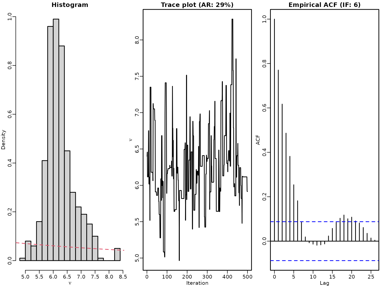
Section 8.3.4 Regression analysis with autocorrelated errors
We begin by loading the data and visualizing them as a time series plot. In what is to follow, we restrict our analysis to the years 2003 through 2012, i.e., a time span of 10 years or 120 observations.
data("newcars", package = "BayesianLearningCode")
newcars <- window(newcars, start = 2003, end = c(2012, 12))
plot(newcars)
Seasonal patterns are evident, as is a trend. To model this, we set
up an appropriate design matrix. Leveraging the fact the the data is a
ts object, we can do this very easily using
time and cycle. Note that
model.matrix will, by default, use the first month
(January) as a baseline and automatically include an intercept.
degree <- 2
tim <- time(newcars)
month <- factor(cycle(tim))
X <- model.matrix(~ month + poly(tim, degree))
head(X)
#>   (Intercept) month2 month3 month4 month5 month6 month7 month8 month9 month10
#> 1           1      0      0      0      0      0      0      0      0       0
#> 2           1      1      0      0      0      0      0      0      0       0
#> 3           1      0      1      0      0      0      0      0      0       0
#> 4           1      0      0      1      0      0      0      0      0       0
#> 5           1      0      0      0      1      0      0      0      0       0
#> 6           1      0      0      0      0      1      0      0      0       0
#>   month11 month12 poly(tim, degree)1 poly(tim, degree)2
#> 1       0       0         -0.1568017          0.1990840
#> 2       0       0         -0.1541664          0.1890461
#> 3       0       0         -0.1515311          0.1791784
#> 4       0       0         -0.1488957          0.1694808
#> 5       0       0         -0.1462604          0.1599534
#> 6       0       0         -0.1436251          0.1505961
d <- ncol(X)
Before including an autoregressive parameter, we first fit a standard regression model, where we assume that the residuals are uncorrelated.
y <- newcars
# Define the burnin and the number of draws thereafter
burnin <- 100
M <- 1000 / mcmcspeedup

# Define the prior parameters
b0 <- rep(0, d)
B0inv <- diag(0, d)
c0 <- 0
C0 <- 0

# Pre-compute some quantities for the Gibbs sampler
XX <- crossprod(X)
Xy <- crossprod(X, y)
cN <- c0 + length(y) / 2

# Allocate space to store the results
betas <- matrix(NA_real_, nrow = M, ncol = d)
colnames(betas) <- colnames(X)
sigma2s <- rep(NA_real_,  M)

# Set the starting values
sigma2 <- var(y) / 2

for (m in 1:(burnin + M)) {
  # Sample beta from its full conditional
  BN <- solve(B0inv + XX / sigma2)
  bN <- BN %*% (B0inv %*% b0 + Xy / sigma2)
  beta <- t(mvtnorm::rmvnorm(1, mean = bN, sigma = BN))

  # Sample sigma^2 from its full conditional
  eps <- y - X %*% beta
  CN <- C0 + crossprod(eps) / 2
  sigma2 <- rinvgamma(1, cN, CN)

  # Store the results
  if (m > burnin) {
    betas[m - burnin, ] <- beta
    sigma2s[m - burnin] <- sigma2
  }
}
We can compute draws of the predicted values and the residuals.
ypreds <- tcrossprod(X, betas)
resids <- as.numeric(y) - ypreds
We proceed with visualizing the data and the mean of the predicted values as well as the mean of the residuals and their estimated ACF.
plot(y, xlab = "Year", ylab = "", main = "New car registrations")
points(tim, rowMeans(ypreds), col = 2, type = 'l')
legend("topleft", c("Data", "Posterior mean"), lty = 1, col = 1:2)
plot(as.numeric(tim), rowMeans(resids), type = 'l', main = "Mean residuals",
     xlab = "Year", ylab = "")
abline(h = 0, lty = 3)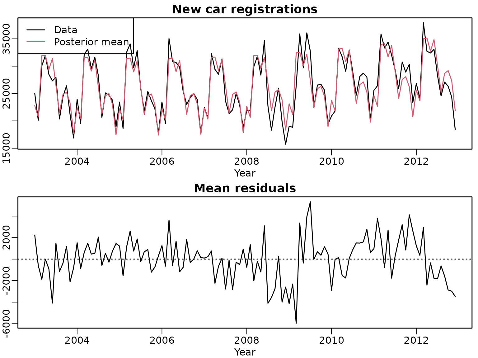
We see a generally good fit but also notice some potential autocorrelation. Thus, we move forward by including an autoregressive coefficient.
# Define the prior parameters for phi (the other ones stay the same)
phiMean <- 0
phiPrec <- 0

# Allocate space to store the results
betas <- matrix(NA_real_, nrow = M, ncol = d)
colnames(betas) <- colnames(X)
sigma2s <- rep(NA_real_,  M)
phis <- rep(NA_real_, M)

# Set the starting values
sigma2 <- var(y) / 2
phi <- 0

for (m in 1:(burnin + M)) {
  # Compute the transformed X and y
  ytilde <- y[-1] - phi * y[-length(y)]
  Xtilde <- X[-1, ] - phi * X[-nrow(X), ]

  # Sample beta from its full conditional
  XX <- crossprod(Xtilde)
  Xy <- crossprod(Xtilde, ytilde)
  BN <- solve(B0inv + XX / sigma2)
  bN <- BN %*% (B0inv %*% b0 + Xy / sigma2)
  beta <- t(mvtnorm::rmvnorm(1, mean = bN, sigma = BN))

  # Compute the errors
  u <- y - X %*% beta

  # Sample sigma^2 from its full conditional
  eps <- u[-1] - phi * u[-length(u)]
  cN <- c0 + length(eps) / 2
  CN <- C0 + crossprod(eps) / 2
  sigma2 <- rinvgamma(1, cN, CN)

  # Sample phi from its full conditional
  XX <- sum(u[-length(u)]^2)
  Xy <- sum(u[-length(u)] * u[-1])
  BN <- 1 / (phiPrec + XX / sigma2)
  bN <- BN * (phiPrec * phiMean + Xy / sigma2)
  phi <- rnorm(1, bN, sqrt(BN))

  # Store the results
  if (m > burnin) {
    betas[m - burnin, ] <- beta
    sigma2s[m - burnin] <- sigma2
    phis[m - burnin] <- phi
  }
}
knitr::kable(c(mean = mean(phis), sd = sd(phis), pos_prob = mean(phis > 0)),
digits = 3, col.names = "phi")| phi | |
|---|---|
| mean | 0.256 |
| sd | 0.110 |
| pos_prob | 0.990 |
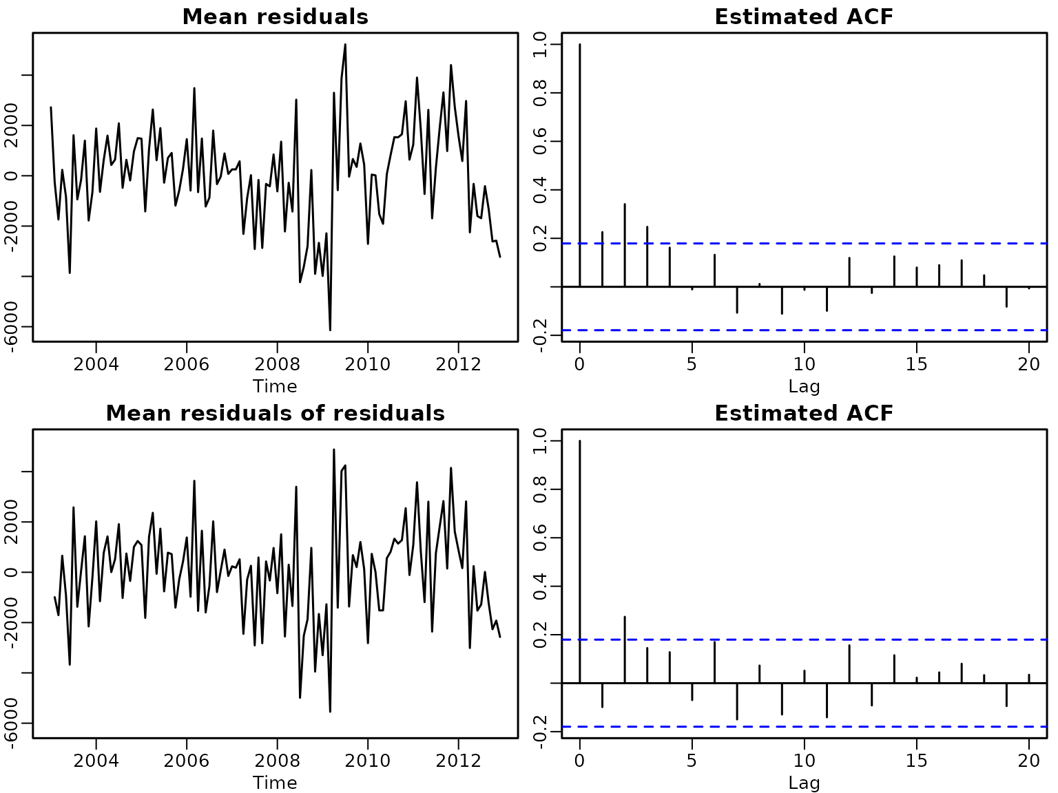
We can again compute draws of the predicted values and the residuals.
preds <- tcrossprod(X, betas)
us <- as.numeric(y) - preds
epss <- us[-1, ] - t(phis * t(us[-nrow(us), ]))
myylim <- range(rowMeans(us), rowMeans(epss))
plot(as.numeric(tim), rowMeans(us), type = "l", xlab = "Time",
     main = "Mean residuals", ylim = myylim)
acf(rowMeans(us))
title("Estimated ACF")
plot(as.numeric(tim), c(NA, rowMeans(epss)), type = "l", xlab = "Time",
     main = "Mean residuals of residuals", ylim = myylim)
acf(rowMeans(epss))
title("Estimated ACF")