Graphical Summary of the Posterior Distribution

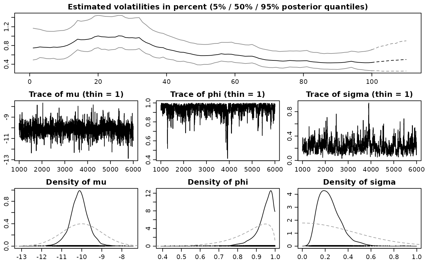
plot.svdraws and plot.svldraws generate some plots visualizing the posterior distribution and can also be used to display predictive distributions of future volatilities.

# S3 method for svdraws
plot(
  x,
  forecast = NULL,
  dates = NULL,
  show0 = FALSE,
  showobs = TRUE,
  showprior = TRUE,
  forecastlty = NULL,
  tcl = -0.4,
  mar = c(1.9, 1.9, 1.7, 0.5),
  mgp = c(2, 0.6, 0),
  simobj = NULL,
  newdata = NULL,
  ...
)

Arguments

x

svdraws object.

forecast

nonnegative integer or object of class svpredict, as returned by predict.svdraws. If an integer greater than 0 is provided, predict.svdraws is invoked to obtain the forecast-step-ahead prediction. The default value is 0.

dates

vector of length ncol(x$latent), providing optional dates for labelling the x-axis. The default value is NULL; in this case, the axis will be labelled with numbers.

show0

logical value, indicating whether the initial volatility exp(h_0/2) should be displayed. The default value is FALSE. Only available for inputs x of class svdraws.

showobs

logical value, indicating whether the observations should be displayed along the x-axis. If many draws have been obtained, the default (TRUE) can render the plotting to be quite slow, and you might want to try setting showobs to FALSE.

showprior

logical value, indicating whether the prior distribution should be displayed. The default value is TRUE.

forecastlty

vector of line type values (see par) used for plotting quantiles of predictive distributions. The default value NULL results in dashed lines.

tcl

The length of tick marks as a fraction of the height of a line of text. See par for details. The default value is -0.4, which results in slightly shorter tick marks than usual.

mar

numerical vector of length 4, indicating the plot margins. See par for details. The default value is c(1.9, 1.9, 1.9, 0.5), which is slightly smaller than the R-defaults.

mgp

numerical vector of length 3, indicating the axis and label positions. See par for details. The default value is c(2, 0.6, 0), which is slightly smaller than the R-defaults.

simobj

object of class svsim as returned by the SV simulation function svsim. If provided, the ``true'' data generating values will be added to the plots.

newdata

corresponds to parameter newdata in predict.svdraws. Only if forecast is a positive integer and predict.svdraws needs a newdata object. Corresponds to input parameter designmatrix in svsample. A matrix of regressors with number of rows equal to parameter forecast.

...

further arguments are passed on to the invoked plotting functions.

Value

Called for its side effects. Returns argument x invisibly.

Details

These functions set up the page layout and call volplot, paratraceplot and paradensplot.

Note

In case you want different quantiles to be plotted, use updatesummary on the svdraws object first. An example of doing so is given in the Examples section.

See also

updatesummary, predict.svdraws

Other plotting: paradensplot(), paratraceplot.svdraws(), paratraceplot(), plot.svpredict(), volplot()

Author

Gregor Kastner gregor.kastner@wu.ac.at

Examples

## Simulate a short and highly persistent SV process
sim <- svsim(100, mu = -10, phi = 0.99, sigma = 0.2)

## Obtain 5000 draws from the sampler (that's not a lot)
draws <- svsample(sim$y, draws = 5000, burnin = 1000,
  priormu = c(-10, 1), priorphi = c(20, 1.5), priorsigma = 0.2)
#> Done!
#> Summarizing posterior draws...

## Plot the latent volatilities and some forecasts
plot(draws, forecast = 10)


## Re-plot with different quantiles
newquants <- c(0.01, 0.05, 0.25, 0.5, 0.75, 0.95, 0.99)
draws <- updatesummary(draws, quantiles = newquants)

plot(draws, forecast = 20, showobs = FALSE,
     forecastlty = 3, showprior = FALSE)