Creates or updates a summary of an svdraws object.
updatesummary(
  x,
  quantiles = c(0.05, 0.5, 0.95),
  esspara = TRUE,
  esslatent = FALSE
)
Arguments
- x
svdrawsobject.- quantiles
numeric vector of posterior quantiles to be computed. The default is
c(0.05, 0.5, 0.95).- esspara
logical value which indicates whether the effective sample size (ESS) should be calculated for the parameter draws. This is achieved by calling
effectiveSizefrom thecodapackage. The default isTRUE.- esslatent
logical value which indicates whether the effective sample size (ESS) should be calculated for the latent log-volatility draws. This is achieved by calling
effectiveSizefrom thecodapackage. The default isFALSE, because this can be quite time-consuming when many latent variables are present.
Value
The value returned is an updated list object of class svdraws
holding
- para
mcmcobject containing the parameter draws from the posterior distribution.- latent
mcmcobject containing the latent instantaneous log-volatility draws from the posterior distribution.- latent0
mcmcobject containing the latent initial log-volatility draws from the posterior distribution.- y
argument
y.- runtime
"proc_time"object containing the run time of the sampler.- priors
listcontaining the parameter values of the prior distribution, i.e. the argumentspriormu,priorphi,priorsigma(and potentiallynu).- thinning
listcontaining the thinning parameters, i.e. the argumentsthinpara,thinlatentandkeeptime.- summary
listcontaining a collection of summary statistics of the posterior draws forpara,latent, andlatent0.
To display the output, use print, summary and plot. The
print method simply prints the posterior draws (which is very likely
a lot of output); the summary method displays the summary statistics
currently stored in the object; the plot method gives a graphical
overview of the posterior distribution by calling volplot,
traceplot and densplot and displaying the
results on a single page.
Details
updatesummary will always calculate the posterior mean and the
posterior standard deviation of the raw draws and some common
transformations thereof. Moroever, the posterior quantiles, specified by the
argument quantiles, are computed. If esspara and/or
esslatent are TRUE, the corresponding effective sample size
(ESS) will also be included.
Note
updatesummary does not actually overwrite the object's current
summary, but in fact creates a new object with an updated summary. Thus,
don't forget to overwrite the old object if this is want you intend to do.
See the examples below for more details.
See also
Examples
## Here is a baby-example to illustrate the idea.
## Simulate an SV time series of length 51 with default parameters:
sim <- svsim(51)
## Draw from the posterior:
res <- svsample(sim$y, draws = 2000, priorphi = c(10, 1.5))
#> Done!
#> Summarizing posterior draws...
## Check out the results:
summary(res)
#>
#> Summary of 'svdraws' object
#>
#> Prior distributions:
#> mu ~ Normal(mean = 0, sd = 100)
#> (phi+1)/2 ~ Beta(a = 10, b = 1.5)
#> sigma^2 ~ Gamma(shape = 0.5, rate = 0.5)
#> nu ~ Infinity
#> rho ~ Constant(value = 0)
#>
#> Stored 2000 MCMC draws after a burn-in of 1000.
#> No thinning.
#>
#> Posterior draws of SV parameters (thinning = 1):
#> mean sd 5% 50% 95% ESS
#> mu -9.82 1.20 -11.1191 -9.8577 -8.621 366
#> phi 0.82 0.16 0.4939 0.8687 0.980 111
#> sigma 0.57 0.22 0.2498 0.5492 0.962 134
#> exp(mu/2) 0.24 7.32 0.0039 0.0072 0.013 366
#> sigma^2 0.37 0.29 0.0624 0.3016 0.926 134
#>
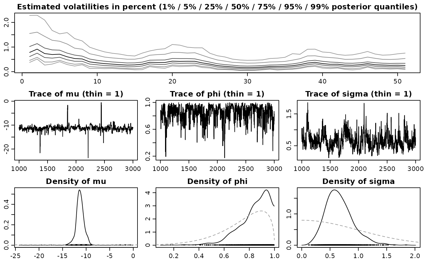
plot(res)
 ## Look at other quantiles and calculate ESS of latents:
newquants <- c(0.01, 0.05, 0.25, 0.5, 0.75, 0.95, 0.99)
res <- updatesummary(res, quantiles = newquants, esslatent = TRUE)
## See the difference?
summary(res)
#>
#> Summary of 'svdraws' object
#>
#> Prior distributions:
#> mu ~ Normal(mean = 0, sd = 100)
#> (phi+1)/2 ~ Beta(a = 10, b = 1.5)
#> sigma^2 ~ Gamma(shape = 0.5, rate = 0.5)
#> nu ~ Infinity
#> rho ~ Constant(value = 0)
#>
#> Stored 2000 MCMC draws after a burn-in of 1000.
#> No thinning.
#>
#> Posterior draws of SV parameters (thinning = 1):
#> mean sd 1% 5% 25% 50% 75% 95% 99%
#> mu -9.82 1.20 -12.3058 -11.1191 -10.2689 -9.8577 -9.5048 -8.621 -7.01
#> phi 0.82 0.16 0.2592 0.4939 0.7595 0.8687 0.9297 0.980 1.00
#> sigma 0.57 0.22 0.1665 0.2498 0.4006 0.5492 0.7047 0.962 1.15
#> exp(mu/2) 0.24 7.32 0.0021 0.0039 0.0059 0.0072 0.0086 0.013 0.03
#> sigma^2 0.37 0.29 0.0277 0.0624 0.1604 0.3016 0.4966 0.926 1.32
#> ESS
#> mu 366
#> phi 111
#> sigma 134
#> exp(mu/2) 366
#> sigma^2 134
#>
plot(res)
## Look at other quantiles and calculate ESS of latents:
newquants <- c(0.01, 0.05, 0.25, 0.5, 0.75, 0.95, 0.99)
res <- updatesummary(res, quantiles = newquants, esslatent = TRUE)
## See the difference?
summary(res)
#>
#> Summary of 'svdraws' object
#>
#> Prior distributions:
#> mu ~ Normal(mean = 0, sd = 100)
#> (phi+1)/2 ~ Beta(a = 10, b = 1.5)
#> sigma^2 ~ Gamma(shape = 0.5, rate = 0.5)
#> nu ~ Infinity
#> rho ~ Constant(value = 0)
#>
#> Stored 2000 MCMC draws after a burn-in of 1000.
#> No thinning.
#>
#> Posterior draws of SV parameters (thinning = 1):
#> mean sd 1% 5% 25% 50% 75% 95% 99%
#> mu -9.82 1.20 -12.3058 -11.1191 -10.2689 -9.8577 -9.5048 -8.621 -7.01
#> phi 0.82 0.16 0.2592 0.4939 0.7595 0.8687 0.9297 0.980 1.00
#> sigma 0.57 0.22 0.1665 0.2498 0.4006 0.5492 0.7047 0.962 1.15
#> exp(mu/2) 0.24 7.32 0.0021 0.0039 0.0059 0.0072 0.0086 0.013 0.03
#> sigma^2 0.37 0.29 0.0277 0.0624 0.1604 0.3016 0.4966 0.926 1.32
#> ESS
#> mu 366
#> phi 111
#> sigma 134
#> exp(mu/2) 366
#> sigma^2 134
#>
plot(res)