Markov Chain Monte Carlo (MCMC) Sampling for the Stochastic Volatility (SV) Model
Source:R/wrappers.R
svsample.Rdsvsample simulates from the joint posterior distribution of the SV
parameters mu, phi, sigma (and potentially nu and rho),
along with the latent log-volatilities h_0,...,h_n and returns the
MCMC draws. If a design matrix is provided, simple Bayesian regression can
also be conducted. For similar functionality with a formula interface,
see svlm.
svsample(
  y,
  draws = 10000,
  burnin = 1000,
  designmatrix = NA,
  priormu = c(0, 100),
  priorphi = c(5, 1.5),
  priorsigma = 1,
  priornu = 0,
  priorrho = NA,
  priorbeta = c(0, 10000),
  priorlatent0 = "stationary",
  priorspec = NULL,
  thin = 1,
  thinpara = thin,
  thinlatent = thin,
  keeptime = "all",
  quiet = FALSE,
  startpara = NULL,
  startlatent = NULL,
  parallel = c("no", "multicore", "snow"),
  n_cpus = 1L,
  cl = NULL,
  n_chains = 1L,
  print_progress = "automatic",
  expert = NULL,
  ...
)

svtsample(
  y,
  draws = 10000,
  burnin = 1000,
  designmatrix = NA,
  priormu = c(0, 100),
  priorphi = c(5, 1.5),
  priorsigma = 1,
  priornu = 0.1,
  priorrho = NA,
  priorbeta = c(0, 10000),
  priorlatent0 = "stationary",
  priorspec = NULL,
  thin = 1,
  thinpara = thin,
  thinlatent = thin,
  keeptime = "all",
  quiet = FALSE,
  startpara = NULL,
  startlatent = NULL,
  parallel = c("no", "multicore", "snow"),
  n_cpus = 1L,
  cl = NULL,
  n_chains = 1L,
  print_progress = "automatic",
  expert = NULL,
  ...
)

svlsample(
  y,
  draws = 20000,
  burnin = 2000,
  designmatrix = NA,
  priormu = c(0, 100),
  priorphi = c(5, 1.5),
  priorsigma = 1,
  priornu = 0,
  priorrho = c(4, 4),
  priorbeta = c(0, 10000),
  priorlatent0 = "stationary",
  priorspec = NULL,
  thin = 1,
  thinpara = thin,
  thinlatent = thin,
  keeptime = "all",
  quiet = FALSE,
  startpara = NULL,
  startlatent = NULL,
  parallel = c("no", "multicore", "snow"),
  n_cpus = 1L,
  cl = NULL,
  n_chains = 1L,
  print_progress = "automatic",
  expert = NULL,
  ...
)

svtlsample(
  y,
  draws = 20000,
  burnin = 2000,
  designmatrix = NA,
  priormu = c(0, 100),
  priorphi = c(5, 1.5),
  priorsigma = 1,
  priornu = 0.1,
  priorrho = c(4, 4),
  priorbeta = c(0, 10000),
  priorlatent0 = "stationary",
  priorspec = NULL,
  thin = 1,
  thinpara = thin,
  thinlatent = thin,
  keeptime = "all",
  quiet = FALSE,
  startpara = NULL,
  startlatent = NULL,
  parallel = c("no", "multicore", "snow"),
  n_cpus = 1L,
  cl = NULL,
  n_chains = 1L,
  print_progress = "automatic",
  expert = NULL,
  ...
)

svsample2(
  y,
  draws = 10000,
  burnin = 1000,
  designmatrix = NA,
  priormu = c(0, 100),
  priorphi = c(5, 1.5),
  priorsigma = 1,
  priornu = 0,
  priorrho = NA,
  priorbeta = c(0, 10000),
  priorlatent0 = "stationary",
  thinpara = 1,
  thinlatent = 1,
  keeptime = "all",
  quiet = FALSE,
  startpara = NULL,
  startlatent = NULL
)
Arguments
- y
numeric vector containing the data (usually log-returns), which must not contain zeros. Alternatively,
ycan be ansvsimobject. In this case, the returns will be extracted and a message is signalled.- draws
single number greater or equal to 1, indicating the number of draws after burn-in (see below). Will be automatically coerced to integer. The default value is 10000.
- burnin
single number greater or equal to 0, indicating the number of draws discarded as burn-in. Will be automatically coerced to integer. The default value is 1000.
- designmatrix
regression design matrix for modeling the mean. Must have
length(y)rows. Alternatively,designmatrixmay be a string of the form"arX", whereXis a nonnegative integer. To fit a constant mean model, usedesignmatrix = "ar0"(which is equivalent todesignmatrix = matrix(1, nrow = length(y))). To fit an AR(1) model, usedesignmatrix = "ar1", and so on. If some elements ofdesignmatrixareNA, the mean is fixed to zero (pre-1.2.0 behavior of stochvol).- priormu
numeric vector of length 2, indicating mean and standard deviation for the Gaussian prior distribution of the parameter
mu, the level of the log-volatility. The default value isc(0, 100), which constitutes a practically uninformative prior for common exchange rate datasets, stock returns and the like.- priorphi
numeric vector of length 2, indicating the shape parameters for the Beta prior distribution of the transformed parameter
(phi + 1) / 2, wherephidenotes the persistence of the log-volatility. The default value isc(5, 1.5), which constitutes a prior that puts some belief in a persistent log-volatility but also encompasses the region wherephiis around 0.- priorsigma
single positive real number, which stands for the scaling of the transformed parameter
sigma^2, wheresigmadenotes the volatility of log-volatility. More precisely,sigma^2 ~ priorsigma * chisq(df = 1). The default value is1, which constitutes a reasonably vague prior for many common exchange rate datasets, stock returns and the like.- priornu
single non-negative number, indicating the rate parameter for the exponential prior distribution of the parameter; can be
Infnu, the degrees-of-freedom parameter of the conditional innovations t-distribution. The default value is0, fixing the degrees-of-freedom to infinity. This corresponds to conditional standard normal innovations, the pre-1.1.0 behavior of stochvol.- priorrho
either
NAfor the no-leverage case or a numeric vector of length 2 that specify the beta prior distribution for(rho+1)/2- priorbeta
numeric vector of length 2, indicating the mean and standard deviation of the Gaussian prior for the regression parameters. The default value is
c(0, 10000), which constitutes a very vague prior for many common datasets. Not used ifdesignmatrixisNA.- priorlatent0
either a single non-negative number or the string
'stationary'(the default, also the behavior before version 1.3.0). Whenpriorlatent0is equal to'stationary', the stationary distribution of the latent AR(1)-process is used as the prior for the initial log-volatilityh_0. Whenpriorlatent0is equal to a number \(B\), we have \(h_0 \sim N(\mu, B\sigma^2)\) a priori.- priorspec
in case one needs different prior distributions than the ones specified by
priormu,...,priorrho, apriorspecobject can be supplied here. A smart constructor for this usecase is specify_priors.- thin
single number greater or equal to 1, coercible to integer. Every
thinparath parameter and latent draw is kept and returned. The default value is 1, corresponding to no thinning of the parameter draws i.e. every draw is stored.- thinpara
single number greater or equal to 1, coercible to integer. Every
thinparath parameter draw is kept and returned. The default value isthin.- thinlatent
single number greater or equal to 1, coercible to integer. Every
thinlatentth latent variable draw is kept and returned. The default value isthin- keeptime
Either 'all' (the default) or 'last'. Indicates which latent volatility draws should be stored.
- quiet
logical value indicating whether the progress bar and other informative output during sampling should be omitted. The default value is
FALSE, implying verbose output.- startpara
optional named list, containing the starting values for the parameter draws. If supplied,
startparamay contain elements namedmu,phi,sigma,nu,rho,beta, andlatent0. The default value is equal to the prior mean. In case of parallel execution withclprovided,startparacan be a list of named lists that initialize the parallel chains.- startlatent
optional vector of length
length(y), containing the starting values for the latent log-volatility draws. The default value isrep(-10, length(y)). In case of parallel execution withclprovided,startlatentcan be a list of numeric vectors that initialize the parallel chains.- parallel
optional one of
"no"(default),"multicore", or"snow", indicating what type of parallellism is to be applied. Option"multicore"is not available on Windows.- n_cpus
optional positive integer, the number of CPUs to be used in case of parallel computations. Defaults to
1L. Ignored if parameterclis supplied andparallel != "snow".- cl
optional so-called SNOW cluster object as implemented in package
parallel. Ignored unlessparallel == "snow".- n_chains
optional positive integer specifying the number of independent MCMC chains
- print_progress
optional one of
"automatic","progressbar", or"iteration", controls the output. Ignored ifquietisTRUE.- expert
optional named list of expert parameters. For most applications, the default values probably work best. Interested users are referred to the literature provided in the References section. If
expertis provided, it may contain the following named elements:- interweave
Logical value. If
TRUE(the default), then ancillarity-sufficiency interweaving strategy (ASIS) is applied to improve on the sampling efficiency for the parameters. Otherwise one parameterization is used.- correct_model_misspecification
Logical value. If
FALSE(the default), then auxiliary mixture sampling is used to sample the latent states. IfTRUE, extra computations are made to correct for model misspecification either ex-post by reweighting or on-line using a Metropolis-Hastings step.
- ...
Any extra arguments will be forwarded to
updatesummary, controlling the type of statistics calculated for the posterior draws.
Value
The value returned is a list object of class svdraws holding
- para
mcmc.listobject containing the parameter draws from the posterior distribution.- latent
mcmc.listobject containing the latent instantaneous log-volatility draws from the posterior distribution.- latent0
mcmc.listobject containing the latent initial log-volatility draws from the posterior distribution.- tau
mcmc.listobject containing the latent variance inflation factors for the sampler with conditional t-innovations (optional).- beta
mcmc.listobject containing the regression coefficient draws from the posterior distribution (optional).- y
the left hand side of the observation equation, usually the argument
y. In case of an AR(k) specification, the firstkelements are removed.- runtime
proc_timeobject containing the run time of the sampler.- priors
a
priorspecobject containing the parameter values of the prior distributions formu,phi,sigma,nu,rho, andbetas, and the variance of specification forlatent0.- thinning
listcontaining the thinning parameters, i.e. the argumentsthinpara,thinlatentandkeeptime.- summary
listcontaining a collection of summary statistics of the posterior draws forpara,latent, andlatent0.- meanmodel
charactercontaining information about howdesignmatrixwas employed.
To display the output, use print, summary and plot. The
print method simply prints the posterior draws (which is very likely
a lot of output); the summary method displays the summary statistics
currently stored in the object; the plot method
plot.svdraws gives a graphical overview of the posterior
distribution by calling volplot, traceplot and
densplot and displaying the results on a single page.
Details
Functions svtsample, svlsample, and svtlsample are
wrappers around svsample with convenient default values for the SV
model with t-errors, leverage, and both t-errors and leverage, respectively.
For details concerning the algorithm please see the paper by Kastner and Frühwirth-Schnatter (2014) and Hosszejni and Kastner (2019).
Note
If y contains zeros, you might want to consider de-meaning your
returns or use designmatrix = "ar0".
svsample2 is deprecated.
References
Kastner, G. and Frühwirth-Schnatter, S. (2014). Ancillarity-sufficiency interweaving strategy (ASIS) for boosting MCMC estimation of stochastic volatility models. Computational Statistics & Data Analysis, 76, 408–423, doi:10.1016/j.csda.2013.01.002 .
Hosszejni, D. and Kastner, G. (2019). Approaches Toward the Bayesian Estimation of the Stochastic Volatility Model with Leverage. Springer Proceedings in Mathematics & Statistics, 296, 75–83, doi:10.1007/978-3-030-30611-3_8 .
See also
Examples
###############
# Full examples
###############
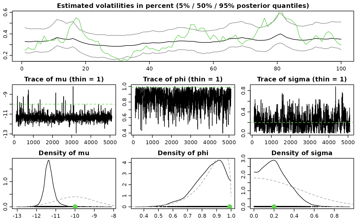
# Example 1
## Simulate a short and highly persistent SV process
sim <- svsim(100, mu = -10, phi = 0.99, sigma = 0.2)
## Obtain 5000 draws from the sampler (that's not a lot)
draws <-
svsample(sim, draws = 5000, burnin = 100,
priormu = c(-10, 1), priorphi = c(20, 1.5), priorsigma = 0.2)
#> Extracted data vector from 'svsim'-object.
#> Done!
#> Summarizing posterior draws...
## Check out the results
summary(draws)
#>
#> Summary of 'svdraws' object
#>
#> Prior distributions:
#> mu ~ Normal(mean = -10, sd = 1)
#> (phi+1)/2 ~ Beta(a = 20, b = 1.5)
#> sigma^2 ~ Gamma(shape = 0.5, rate = 2.5)
#> nu ~ Infinity
#> rho ~ Constant(value = 0)
#>
#> Stored 5000 MCMC draws after a burn-in of 100.
#> No thinning.
#>
#> Posterior draws of SV parameters (thinning = 1):
#> mean sd 5% 50% 95% ESS
#> mu -10.1400 0.23657 -1.0e+01 -10.1445 -9.7614 999
#> phi 0.8455 0.10712 6.4e-01 0.8676 0.9781 470
#> sigma 0.1616 0.11700 1.5e-02 0.1416 0.3759 355
#> exp(mu/2) 0.0063 0.00077 5.3e-03 0.0063 0.0076 999
#> sigma^2 0.0398 0.05906 2.4e-04 0.0200 0.1413 355
#>
plot(draws)
#> Simulation object extracted from input
 # \donttest{
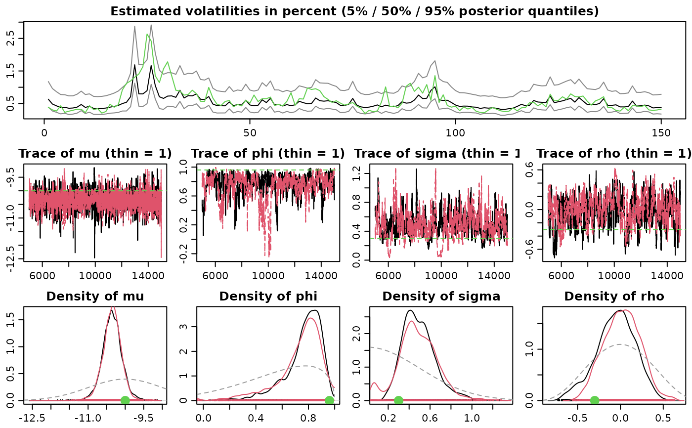
# Example 2
## Simulate an asymmetric and conditionally heavy-tailed SV process
sim <- svsim(150, mu = -10, phi = 0.96, sigma = 0.3, nu = 10, rho = -0.3)
## Obtain 10000 draws from the sampler
## Use more advanced prior settings
## Run two parallel MCMC chains
advanced_draws <-
svsample(sim, draws = 10000, burnin = 5000,
priorspec = specify_priors(mu = sv_normal(-10, 1),
sigma2 = sv_gamma(0.5, 2),
rho = sv_beta(4, 4),
nu = sv_constant(5)),
parallel = "snow", n_chains = 2, n_cpus = 2)
#> Extracted data vector from 'svsim'-object.
#> Done!
#> Summarizing posterior draws...
## Check out the results
summary(advanced_draws)
#>
#> Summary of 'svdraws' object
#>
#> Prior distributions:
#> mu ~ Normal(mean = -10, sd = 1)
#> (phi+1)/2 ~ Beta(a = 5, b = 1.5)
#> sigma^2 ~ Gamma(shape = 0.5, rate = 2)
#> nu ~ Constant(value = 5)
#> rho ~ Beta(a = 4, b = 4)
#>
#> Stored 10000 MCMC draws after a burn-in of 5000.
#> No thinning.
#>
#> Posterior draws of SV parameters (thinning = 1):
#> mean sd 5% 50% 95% ESS
#> mu -9.8968 0.5676 -10.8475 -9.8698 -9.017 2561
#> phi 0.9314 0.0385 0.8574 0.9382 0.982 455
#> sigma 0.4948 0.1211 0.3093 0.4884 0.707 233
#> rho -0.3157 0.1648 -0.5679 -0.3275 -0.028 406
#> exp(mu/2) 0.0074 0.0021 0.0044 0.0072 0.011 2561
#> sigma^2 0.2595 0.1277 0.0956 0.2386 0.499 233
#>
plot(advanced_draws)
#> Simulation object extracted from input
# \donttest{
# Example 2
## Simulate an asymmetric and conditionally heavy-tailed SV process
sim <- svsim(150, mu = -10, phi = 0.96, sigma = 0.3, nu = 10, rho = -0.3)
## Obtain 10000 draws from the sampler
## Use more advanced prior settings
## Run two parallel MCMC chains
advanced_draws <-
svsample(sim, draws = 10000, burnin = 5000,
priorspec = specify_priors(mu = sv_normal(-10, 1),
sigma2 = sv_gamma(0.5, 2),
rho = sv_beta(4, 4),
nu = sv_constant(5)),
parallel = "snow", n_chains = 2, n_cpus = 2)
#> Extracted data vector from 'svsim'-object.
#> Done!
#> Summarizing posterior draws...
## Check out the results
summary(advanced_draws)
#>
#> Summary of 'svdraws' object
#>
#> Prior distributions:
#> mu ~ Normal(mean = -10, sd = 1)
#> (phi+1)/2 ~ Beta(a = 5, b = 1.5)
#> sigma^2 ~ Gamma(shape = 0.5, rate = 2)
#> nu ~ Constant(value = 5)
#> rho ~ Beta(a = 4, b = 4)
#>
#> Stored 10000 MCMC draws after a burn-in of 5000.
#> No thinning.
#>
#> Posterior draws of SV parameters (thinning = 1):
#> mean sd 5% 50% 95% ESS
#> mu -9.8968 0.5676 -10.8475 -9.8698 -9.017 2561
#> phi 0.9314 0.0385 0.8574 0.9382 0.982 455
#> sigma 0.4948 0.1211 0.3093 0.4884 0.707 233
#> rho -0.3157 0.1648 -0.5679 -0.3275 -0.028 406
#> exp(mu/2) 0.0074 0.0021 0.0044 0.0072 0.011 2561
#> sigma^2 0.2595 0.1277 0.0956 0.2386 0.499 233
#>
plot(advanced_draws)
#> Simulation object extracted from input
 # Example 3
## AR(1) structure for the mean
data(exrates)
len <- 3000
ahead <- 100
y <- head(exrates$USD, len)
## Fit AR(1)-SVL model to EUR-USD exchange rates
res <- svsample(y, designmatrix = "ar1")
#> Done!
#> Summarizing posterior draws...
## Use predict.svdraws to obtain predictive distributions
preddraws <- predict(res, steps = ahead)
## Calculate predictive quantiles
predquants <- apply(predy(preddraws), 2, quantile, c(.1, .5, .9))
## Visualize
expost <- tail(head(exrates$USD, len+ahead), ahead)
ts.plot(y, xlim = c(length(y)-4*ahead, length(y)+ahead),
ylim = range(c(predquants, expost, tail(y, 4*ahead))))
for (i in 1:3) {
lines((length(y)+1):(length(y)+ahead), predquants[i,],
col = 3, lty = c(2, 1, 2)[i])
}
lines((length(y)+1):(length(y)+ahead), expost,
col = 2)
# Example 3
## AR(1) structure for the mean
data(exrates)
len <- 3000
ahead <- 100
y <- head(exrates$USD, len)
## Fit AR(1)-SVL model to EUR-USD exchange rates
res <- svsample(y, designmatrix = "ar1")
#> Done!
#> Summarizing posterior draws...
## Use predict.svdraws to obtain predictive distributions
preddraws <- predict(res, steps = ahead)
## Calculate predictive quantiles
predquants <- apply(predy(preddraws), 2, quantile, c(.1, .5, .9))
## Visualize
expost <- tail(head(exrates$USD, len+ahead), ahead)
ts.plot(y, xlim = c(length(y)-4*ahead, length(y)+ahead),
ylim = range(c(predquants, expost, tail(y, 4*ahead))))
for (i in 1:3) {
lines((length(y)+1):(length(y)+ahead), predquants[i,],
col = 3, lty = c(2, 1, 2)[i])
}
lines((length(y)+1):(length(y)+ahead), expost,
col = 2)
 # Example 4
## Predicting USD based on JPY and GBP in the mean
data(exrates)
len <- 3000
ahead <- 30
## Calculate log-returns
logreturns <- apply(exrates[, c("USD", "JPY", "GBP")], 2,
function (x) diff(log(x)))
logretUSD <- logreturns[2:(len+1), "USD"]
regressors <- cbind(1, as.matrix(logreturns[1:len, ])) # lagged by 1 day
## Fit SV model to EUR-USD exchange rates
res <- svsample(logretUSD, designmatrix = regressors)
#> Done!
#> Summarizing posterior draws...
## Use predict.svdraws to obtain predictive distributions
predregressors <- cbind(1, as.matrix(logreturns[(len+1):(len+ahead), ]))
preddraws <- predict(res, steps = ahead,
newdata = predregressors)
predprice <- exrates[len+2, "USD"] * exp(t(apply(predy(preddraws), 1, cumsum)))
## Calculate predictive quantiles
predquants <- apply(predprice, 2, quantile, c(.1, .5, .9))
## Visualize
priceUSD <- exrates[3:(len+2), "USD"]
expost <- exrates[(len+3):(len+ahead+2), "USD"]
ts.plot(priceUSD, xlim = c(len-4*ahead, len+ahead+1),
ylim = range(c(expost, predquants, tail(priceUSD, 4*ahead))))
for (i in 1:3) {
lines(len:(len+ahead), c(tail(priceUSD, 1), predquants[i,]),
col = 3, lty = c(2, 1, 2)[i])
}
lines(len:(len+ahead), c(tail(priceUSD, 1), expost),
col = 2)
# Example 4
## Predicting USD based on JPY and GBP in the mean
data(exrates)
len <- 3000
ahead <- 30
## Calculate log-returns
logreturns <- apply(exrates[, c("USD", "JPY", "GBP")], 2,
function (x) diff(log(x)))
logretUSD <- logreturns[2:(len+1), "USD"]
regressors <- cbind(1, as.matrix(logreturns[1:len, ])) # lagged by 1 day
## Fit SV model to EUR-USD exchange rates
res <- svsample(logretUSD, designmatrix = regressors)
#> Done!
#> Summarizing posterior draws...
## Use predict.svdraws to obtain predictive distributions
predregressors <- cbind(1, as.matrix(logreturns[(len+1):(len+ahead), ]))
preddraws <- predict(res, steps = ahead,
newdata = predregressors)
predprice <- exrates[len+2, "USD"] * exp(t(apply(predy(preddraws), 1, cumsum)))
## Calculate predictive quantiles
predquants <- apply(predprice, 2, quantile, c(.1, .5, .9))
## Visualize
priceUSD <- exrates[3:(len+2), "USD"]
expost <- exrates[(len+3):(len+ahead+2), "USD"]
ts.plot(priceUSD, xlim = c(len-4*ahead, len+ahead+1),
ylim = range(c(expost, predquants, tail(priceUSD, 4*ahead))))
for (i in 1:3) {
lines(len:(len+ahead), c(tail(priceUSD, 1), predquants[i,]),
col = 3, lty = c(2, 1, 2)[i])
}
lines(len:(len+ahead), c(tail(priceUSD, 1), expost),
col = 2)
 # }
########################
# Further short examples
########################
y <- svsim(50, nu = 10, rho = -0.1)$y
# Supply initial values
res <- svsample(y,
startpara = list(mu = -10, sigma = 1))
#> Done!
#> Summarizing posterior draws...
# \donttest{
# Supply initial values for parallel chains
res <- svsample(y,
startpara = list(list(mu = -10, sigma = 1),
list(mu = -11, sigma = .1, phi = 0.9),
list(mu = -9, sigma = .3, phi = 0.7)),
parallel = "snow", n_chains = 3, n_cpus = 2)
#> Done!
#> Summarizing posterior draws...
# Parallel chains with with a pre-defined cluster object
cl <- parallel::makeCluster(2, "PSOCK", outfile = NULL) # print to console
res <- svsample(y,
parallel = "snow", n_chains = 3, cl = cl)
#> Done!
#> Summarizing posterior draws...
parallel::stopCluster(cl)
# }
# Turn on correction for model misspecification
## Since the approximate model is fast and it is working very
## well in practice, this is turned off by default
res <- svsample(y,
expert = list(correct_model_misspecification = TRUE))
#> Done!
#> Summarizing posterior draws...
#> No computation of effective sample size after re-sampling
print(res)
#>
#> Summary of 'svdraws' object
#>
#> Prior distributions:
#> mu ~ Normal(mean = 0, sd = 100)
#> (phi+1)/2 ~ Beta(a = 5, b = 1.5)
#> sigma^2 ~ Gamma(shape = 0.5, rate = 0.5)
#> nu ~ Infinity
#> rho ~ Constant(value = 0)
#>
#> Stored 10000 MCMC draws after a burn-in of 1000.
#> No thinning.
#>
#> Posterior draws of SV parameters (thinning = 1):
#> mean sd 5% 50% 95%
#> mu -10.2642 0.5215 -10.9605 -10.226 -9.661
#> phi 0.5703 0.2863 0.0324 0.618 0.940
#> sigma 0.5192 0.2763 0.1077 0.495 1.014
#> exp(mu/2) 0.0061 0.0015 0.0042 0.006 0.008
#> sigma^2 0.3460 0.3468 0.0116 0.245 1.029
#>
#> Posterior draws from the auxiliary SV model were re-sampled after the MCMC
#> procedure ended to correct for model mis-specification.
#> Re-sampling of parameters and latents was of little practical importance:
#> - max reachable entropy for this sample size: 9.21034,
#> - entropy of the re-sampling weight distribution: 9.210184
#>
if (FALSE) { # \dontrun{
# Parallel multicore chains (not available on Windows)
res <- svsample(y, draws = 30000, burnin = 10000,
parallel = "multicore", n_chains = 3, n_cpus = 2)
# Plot using a color palette
palette(rainbow(coda::nchain(para(res, "all"))))
plot(res)
# Use functionality from package 'coda'
## E.g. Geweke's convergence diagnostics
coda::geweke.diag(para(res, "all")[, c("mu", "phi", "sigma")])
# Use functionality from package 'bayesplot'
bayesplot::mcmc_pairs(res, pars = c("sigma", "mu", "phi", "h_0", "h_15"))
} # }
# }
########################
# Further short examples
########################
y <- svsim(50, nu = 10, rho = -0.1)$y
# Supply initial values
res <- svsample(y,
startpara = list(mu = -10, sigma = 1))
#> Done!
#> Summarizing posterior draws...
# \donttest{
# Supply initial values for parallel chains
res <- svsample(y,
startpara = list(list(mu = -10, sigma = 1),
list(mu = -11, sigma = .1, phi = 0.9),
list(mu = -9, sigma = .3, phi = 0.7)),
parallel = "snow", n_chains = 3, n_cpus = 2)
#> Done!
#> Summarizing posterior draws...
# Parallel chains with with a pre-defined cluster object
cl <- parallel::makeCluster(2, "PSOCK", outfile = NULL) # print to console
res <- svsample(y,
parallel = "snow", n_chains = 3, cl = cl)
#> Done!
#> Summarizing posterior draws...
parallel::stopCluster(cl)
# }
# Turn on correction for model misspecification
## Since the approximate model is fast and it is working very
## well in practice, this is turned off by default
res <- svsample(y,
expert = list(correct_model_misspecification = TRUE))
#> Done!
#> Summarizing posterior draws...
#> No computation of effective sample size after re-sampling
print(res)
#>
#> Summary of 'svdraws' object
#>
#> Prior distributions:
#> mu ~ Normal(mean = 0, sd = 100)
#> (phi+1)/2 ~ Beta(a = 5, b = 1.5)
#> sigma^2 ~ Gamma(shape = 0.5, rate = 0.5)
#> nu ~ Infinity
#> rho ~ Constant(value = 0)
#>
#> Stored 10000 MCMC draws after a burn-in of 1000.
#> No thinning.
#>
#> Posterior draws of SV parameters (thinning = 1):
#> mean sd 5% 50% 95%
#> mu -10.2642 0.5215 -10.9605 -10.226 -9.661
#> phi 0.5703 0.2863 0.0324 0.618 0.940
#> sigma 0.5192 0.2763 0.1077 0.495 1.014
#> exp(mu/2) 0.0061 0.0015 0.0042 0.006 0.008
#> sigma^2 0.3460 0.3468 0.0116 0.245 1.029
#>
#> Posterior draws from the auxiliary SV model were re-sampled after the MCMC
#> procedure ended to correct for model mis-specification.
#> Re-sampling of parameters and latents was of little practical importance:
#> - max reachable entropy for this sample size: 9.21034,
#> - entropy of the re-sampling weight distribution: 9.210184
#>
if (FALSE) { # \dontrun{
# Parallel multicore chains (not available on Windows)
res <- svsample(y, draws = 30000, burnin = 10000,
parallel = "multicore", n_chains = 3, n_cpus = 2)
# Plot using a color palette
palette(rainbow(coda::nchain(para(res, "all"))))
plot(res)
# Use functionality from package 'coda'
## E.g. Geweke's convergence diagnostics
coda::geweke.diag(para(res, "all")[, c("mu", "phi", "sigma")])
# Use functionality from package 'bayesplot'
bayesplot::mcmc_pairs(res, pars = c("sigma", "mu", "phi", "h_0", "h_15"))
} # }