All the heavy lifting in stochvol is implemented in C++
with the help of R packages Rcpp and RcppArmadillo.
These functions call the MCMC samplers in C++ directly without any
any validation and transformations, expert use only!
svsample_fast_cpp(
  y,
  draws = 1,
  burnin = 0,
  designmatrix = matrix(NA),
  priorspec = specify_priors(),
  thinpara = 1,
  thinlatent = 1,
  keeptime = "all",
  startpara,
  startlatent,
  keeptau = !inherits(priorspec$nu, "sv_infinity"),
  print_settings = list(quiet = TRUE, n_chains = 1, chain = 1),
  correct_model_misspecification = FALSE,
  interweave = TRUE,
  myoffset = 0,
  fast_sv = get_default_fast_sv()
)

svsample_general_cpp(
  y,
  draws = 1,
  burnin = 0,
  designmatrix = matrix(NA),
  priorspec = specify_priors(),
  thinpara = 1,
  thinlatent = 1,
  keeptime = "all",
  startpara,
  startlatent,
  keeptau = !inherits(priorspec$nu, "sv_infinity"),
  print_settings = list(quiet = TRUE, n_chains = 1, chain = 1),
  correct_model_misspecification = FALSE,
  interweave = TRUE,
  myoffset = 0,
  general_sv = get_default_general_sv(priorspec)
)
Arguments
- y
numeric vector of the observations
- draws
single positive integer, the number of draws to return (after the burn-in)
- burnin
single positive integer, length of warm-up period, this number of draws are discarded from the beginning
- designmatrix
numeric matrix of covariates. Dimensions:
length(y)times the number of covariates. If there are no covariates then this should bematrix(NA)- priorspec
a
priorspecobject created byspecify_priors- thinpara
single number greater or equal to 1, coercible to integer. Every
thinparath parameter draw is kept and returned. The default value is 1, corresponding to no thinning of the parameter draws i.e. every draw is stored.- thinlatent
single number greater or equal to 1, coercible to integer. Every
thinlatentth latent variable draw is kept and returned. The default value is 1, corresponding to no thinning of the latent variable draws, i.e. every draw is kept.- keeptime
Either 'all' (the default) or 'last'. Indicates which latent volatility draws should be stored.
- startpara
named list, containing the starting values for the parameter draws. It must contain elements
mu: an arbitrary numerical value
phi: real number between
-1and1sigma: a positive real number
nu: a number larger than
2; can beInfrho: real number between
-1and1beta: a numeric vector of the same length as the number of covariates
latent0: a single number, the initial value for
h0
- startlatent
vector of length
length(y), containing the starting values for the latent log-volatility draws.- keeptau
Logical value indicating whether the 'variance inflation factors' should be stored (used for the sampler with conditional t innovations only). This may be useful to check at what point(s) in time the normal disturbance had to be 'upscaled' by a mixture factor and when the series behaved 'normally'.
- print_settings
List of three elements:
quiet: logical value indicating whether the progress bar and other informative output during sampling should be omitted
n_chains: number of independent MCMC chains
chain: index of this chain
Please note that this function does not run multiple independent chains but
svsampleoffers different printing functionality depending on whether it is executed as part of several MCMC chains in parallel (chain specific messages) or simply as a single chain (progress bar).- correct_model_misspecification
Logical value. If
FALSE, then auxiliary mixture sampling is used to sample the latent states. IfTRUE, extra computations are made to correct for model misspecification either ex-post by reweighting or on-line using a Metropolis-Hastings step.- interweave
Logical value. If
TRUE, then ancillarity-sufficiency interweaving strategy (ASIS) is applied to improve on the sampling efficiency for the parameters. Otherwise one parameterization is used.- myoffset
Single non-negative number that is used in
log(y^2 + myoffset)to prevent-Infvalues in the auxiliary mixture sampling scheme.- fast_sv
named list of expert settings. We recommend the use of
get_default_fast_sv.- general_sv
named list of expert settings. We recommend the use of
get_default_general_sv.
Details
The sampling functions are separated into fast SV and general SV. See more details in the sections below.
Fast SV
Fast SV was developed in Kastner and Fruehwirth-Schnatter (2014). Fast SV estimates an approximate SV model without leverage, where the approximation comes in through auxiliary mixture approximations to the exact SV model. The sampler uses the ancillarity-sufficiency interweaving strategy (ASIS) to improve on the sampling efficiency of the model parameters, and it employs all-without-a-loop (AWOL) for computationally efficient Kalman filtering of the conditionally Gaussian state space. Correction for model misspecification happens as a post-processing step.
Fast SV employs sampling strategies that have been fine-tuned and specified for
vanilla SV (no leverage), and hence it can be fast and efficient but also more limited
in its feature set. The conditions for the fast SV sampler: rho == 0; mu
has either a normal prior or it is also constant 0; the prior for phi
is a beta distribution; the prior for sigma^2 is either a gamma distribution
with shape 0.5 or a mean- and variance-matched inverse gamma distribution;
either keeptime == 'all' or correct_model_misspecification == FALSE.
These criteria are NOT VALIDATED by fast SV on the C++ level!
General SV
General SV also estimates an approximate SV model without leverage, where the approximation comes in through auxiliary mixture approximations to the exact SV model. The sampler uses both ASIS and AWOL.
General SV employs adapted random walk Metropolis-Hastings as the proposal for
the parameters mu, phi, sigma, and rho. Therefore,
more general prior distributions are allowed in this case.
Examples
# Draw one sample using fast SV and general SV
y <- svsim(40)$y
params <- list(mu = -10, phi = 0.9, sigma = 0.1,
nu = Inf, rho = 0, beta = NA,
latent0 = -10)
res_fast <- svsample_fast_cpp(y,
startpara = params, startlatent = rep(-10, 40))
res_gen <- svsample_general_cpp(y,
startpara = params, startlatent = rep(-10, 40))
# Embed SV in another sampling scheme
## vanilla SV
len <- 40L
draws <- 1000L
burnin <- 200L
param_store <- matrix(NA, draws, 3,
dimnames = list(NULL,
c("mu", "phi", "sigma")))
startpara <- list(mu = 0, phi = 0.9, sigma = 0.1,
nu = Inf, rho = 0, beta = NA,
latent0 = 0)
startlatent <- rep(0, len)
for (i in seq_len(burnin+draws)) {
# draw the data in the bigger sampling scheme
# now we simulate y from vanilla SV
y <- svsim(len, mu = 0, phi = 0.9, sigma = 0.1)$y
# call SV sampler
res <- svsample_fast_cpp(y, startpara = startpara,
startlatent = startlatent)
# administrate values
startpara[c("mu","phi","sigma")] <-
as.list(res$para[, c("mu", "phi", "sigma")])
startlatent <- drop(res$latent)
# store draws after the burnin
if (i > burnin) {
param_store[i-burnin, ] <-
res$para[, c("mu", "phi", "sigma")]
}
}
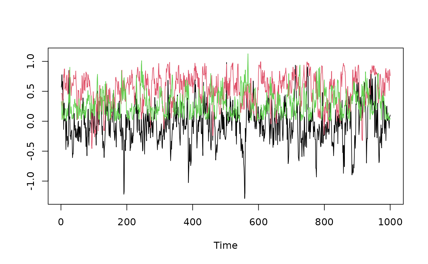
### quick look at the traceplots
ts.plot(param_store, col = 1:3)